Chapter 6 The Link Layer and LANs

There are two fundamentally different types of link-layer channels. The first type are broadcast channels, which connect multiple hosts in wireless LANs, satellite networks, and hybrid fiber-coaxial cable (HFC) access networks. Since many hosts are connected to the same broadcast communication channel, a so-called medium access protocol is needed to coordinate frame transmission. In some cases, a central controller may be used to coordinate transmissions; in other cases, the hosts themselves coordinate transmissions. The second type of link-layer channel is the point-to-point communication link, such as that often found between two routers connected by a long-distance link, or between a user’s office computer and the nearby Ethernet switch to which it is connected.

6.1 Introduction to the Link Layer

6.1.1 The Services Provided by the Link Layer

Although the basic service of any link layer is to move a datagram from one node to an adjacent node over a single communication link, the details of the provided service can vary from one link-layer protocol to the next. Possible services that can be offered by a link-layer protocol include:

• Framing. Almost all link-layer protocols encapsulate each network-layer datagram within a link-layer frame before transmission over the link. A frame consists of a data field, in which the network-layer datagram is inserted, and a number of header fields. The structure of the frame is specified by the link-layer protocol.
• Link access. A medium access control (MAC) protocol specifies the rules by which a frame is transmitted onto the link. For point-to-point links that have a single sender at one end of the link and a single receiver at the other end of the link, the MAC protocol is simple (or nonexistent)—the sender can send a frame whenever the link is idle. The more interesting case is when multiple nodes share a single broadcast link—the so-called multiple access problem. Here, the MAC protocol serves to coordinate the frame transmissions of the many nodes.
• Reliable delivery. When a link-layer protocol provides reliable delivery service, it guarantees to move each network-layer datagram across the link without error. Recall that certain transport-layer protocols (such as TCP) also provide a reliable delivery service. Similar to a transport-layer reliable delivery service, a link-layer reliable delivery service can be achieved with acknowledgments and retransmissions. A link-layer reliable delivery service is often used for links that are prone to high error rates, such as a wireless link, with the goal of correcting an error locally—on the link where the error occurs—rather than forcing an end-to-end retransmission of the data by a transport- or application-layer protocol. However, link-layer reliable delivery can be considered an unnecessary overhead for low bit-error links, including fiber, coax, and many twisted-pair copper links. For this reason, many wired link-layer protocols do not provide a reliable delivery service.
• Error detection and correction. The link-layer hardware in a receiving node can incorrectly decide that a bit in a frame is zero when it was transmitted as a one, and vice versa. Such bit errors are introduced by signal attenuation and electromagnetic noise. Because there is no need to forward a datagram that has an error, many link-layer protocols provide a mechanism to detect such bit errors. This is done by having the transmitting node include error-detection bits in the frame, and having the receiving node perform an error check. The Internet’s transport layer and network layer also provide a limited form of error detection—the Internet checksum. Error detection in the link layer is usually more sophisticated and is implemented in hardware. Error correction is similar to error detection, except that a receiver not only detects when bit errors have occurred in the frame but also determines exactly where in the frame the errors have occurred (and then corrects these errors).

6.1.2 Where Is the Link Layer Implemented?

For the most part, the link layer is implemented in a network adapter, also sometimes known as a network interface card (NIC). At the heart of the network adapter is the link-layer controller, usually a single, special-purpose chip that implements many of the link-layer services (framing, link access, error detection, and so on). Thus, much of a link-layer controller’s functionality is implemented in hardware. Until the late 1990s, most network adapters were physically separate cards (such as a PCMCIA card or a plug-in card fitting into a PC’s PCI card slot) but increasingly, network adapters are being integrated onto the host’s motherboard—a so-called LAN-on-motherboard configuration.

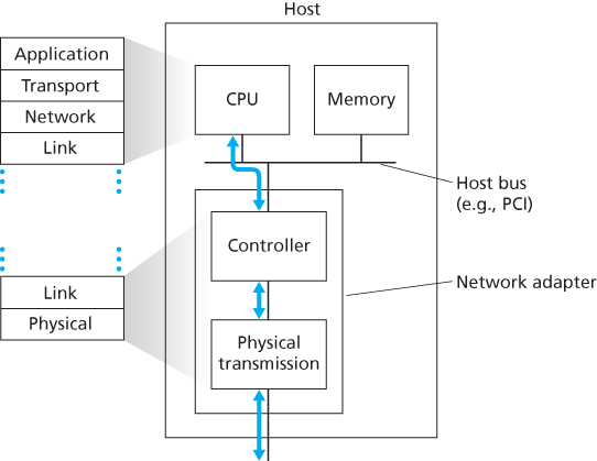
Most of the link layer is implemented in hardware, part of the link layer is implemented in software that runs on the host’s CPU. The software components of the link layer implement higher-level link-layer functionality such as assembling link-layer addressing information and activating the controller hardware. On the receiving side, link-layer software responds to controller interrupts (e.g., due to the receipt of one or more frames), handling error conditions and passing a datagram up to the network layer.

6.2 Error-Detection and -Correction Techniques

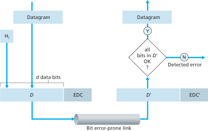
At the sending node, data, D, to be protected against bit errors is augmented with error-detection and -correction bits (EDC). Typically, the data to be protected includes not only the datagram passed down from the network layer for transmission across the link, but also link-level addressing information, sequence numbers, and other fields in the link frame header.

Error-detection and -correction techniques allow the receiver to sometimes, but not always, detect that bit errors have occurred. Even with the use of error-detection bits there still may be undetected bit errors; that is, the receiver may be unaware that the received information contains bit errors.

6.2.1 Parity Checks

In an even parity scheme, the sender simply includes one additional bit and chooses its value such that the total number of 1s in the  bits (the original information plus a parity bit) is even. For odd parity schemes, the parity bit value is chosen such that there is an odd number of 1s.

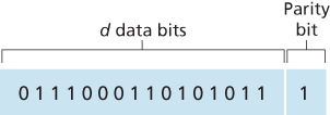
The receiver need only count the number of 1s in the received  bits. If an odd number of 1-valued bits are found with an even parity scheme, the receiver knows that at least one bit error has occurred. More precisely, it knows that some odd number of bit errors have occurred.

The ability of the receiver to both detect and correct errors is known as forward error correction (FEC). These techniques are commonly used in audio storage and playback devices such as audio CDs.

6.2.2 Checksumming Methods

In checksumming techniques, the d bits of data are treated as a sequence of k-bit integers. One simple checksumming method is to simply sum these k-bit integers and use the resulting sum as the error-detection bits. The Internet checksum is based on this approach—bytes of data are treated as 16-bit integers and summed.

6.2.3 Cyclic Redundancy Check (CRC)

CRC codes are also known as polynomial codes, since it is possible to view the bit string to be sent as a polynomial whose coefficients are the 0 and 1 values in the bit string, with operations on the bit string interpreted as polynomial arithmetic.

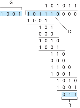
CRC codes operate as follows. Consider the d-bit piece of data, D, that the sending node wants to send to the receiving node. The sender and receiver must first agree on an bit pattern, known as a generator, which we will denote as G. We will require that the most significant (leftmost) bit of G be a 1. For a given piece of data, D, the sender will choose r additional bits, R, and append them to D such that the resulting bit pattern (interpreted as a binary number) is exactly divisible by G (i.e., has no remainder) using modulo-2 arithmetic. The process of error checking with CRCs is thus simple: The receiver divides the  received bits by G. If the remainder is nonzero, the receiver knows that an error has occurred; otherwise the data is accepted as being correct.

All CRC calculations are done in modulo-2 arithmetic without carries in addition or borrows in subtraction. This means that addition and subtraction are identical, and both are equivalent to the bitwise exclusive-or (XOR) of the operands. For example:

1011 XOR 0101 = 1110
1001 XOR 1101 = 0100

Also, we similarly have

1011 - 0101 = 1110
1001 - 1101 = 0100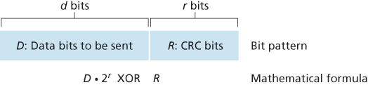

Let us now turn to the crucial question of how the sender computes R. Recall that we want to find R such that there is an n such that

That is, we want to choose R such that G divides into  without remainder. If we XOR (that is, add modulo-2, without carry) R to both sides of the above equation, we get

This equation tells us that if we divide by G, the value of the remainder is precisely R. In other words, we can calculate R as

For the case of , , and . The 9 bits transmitted in this case are 101 110  011.

International standards have been defined for 8-, 12-, 16-, and 32-bit generators, G. The CRC-32 32-bit standard, which has been adopted in a number of link-level IEEE protocols, uses a generator of

Each of the CRC standards can detect burst errors of fewer than bits. This means that all consecutive bit errors of r bits or fewer will be detected. Furthermore, under appropriate assumptions, a burst of length greater than bits is detected with probability . Also, each of the CRC standards can detect any odd number of bit errors.

6.3 Multiple Access Links and Protocols

Multiple access protocols are needed in a wide variety of network settings, including both wired and wireless access networks, and satellite networks. Although technically each node accesses the broadcast channel through its adapter, in this section we will refer to the node as the sending and receiving device. In practice, hundreds or even thousands of nodes can directly communicate over a broadcast channel.

Because all nodes are capable of transmitting frames, more than two nodes can transmit frames at the same time. When this happens, all of the nodes receive multiple frames at the same time; that is, the transmitted frames collide at all of the receivers. Typically, when there is a collision, none of the receiving nodes can make any sense of any of the frames that were transmitted; in a sense, the signals of the colliding frames become inextricably tangled together.

6.3.1 Channel Partitioning Protocols

Time-division multiplexing (TDM) and frequency-division multiplexing (FDM) are two techniques that can be used to partition a broadcast channel’s bandwidth among all nodes sharing that channel.

A third channel partitioning protocol is code division multiple access (CDMA). While TDM and FDM assign time slots and frequencies, respectively, to the nodes, CDMA assigns a different code to each node. Each node then uses its unique code to encode the data bits it sends. If the codes are chosen carefully, CDMA networks have the wonderful property that different nodes can transmit simultaneously and yet have their respective receivers correctly receive a sender’s encoded data bits (assuming the receiver knows the sender’s code) in spite of interfering transmissions by other nodes.

6.3.2 Random Access Protocols

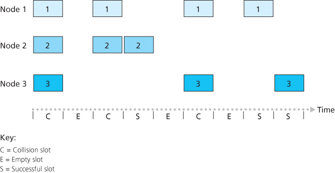
In a random access protocol, a transmitting node always transmits at the full rate of the channel, namely, R bps. When there is a collision, each node involved in the collision repeatedly retransmits its frame (that is, packet) until its frame gets through without a collision. But when a node experiences a collision, it doesn’t necessarily retransmit the frame right away. Instead it waits a random delay before retransmitting the frame. Each node involved in a collision chooses independent random delays. Because the random delays are independently chosen, it is possible that one of the nodes will pick a delay that is sufficiently less than the delays of the other colliding nodes and will therefore be able to sneak its frame into the channel without a collision.

Slotted ALOHA

The operation of slotted ALOHA in each node is simple:

• When the node has a fresh frame to send, it waits until the beginning of the next slot and transmits the entire frame in the slot.
• If there isn’t a collision, the node has successfully transmitted its frame and thus need not consider retransmitting the frame. The node can prepare a new frame for transmission, if it has one.
• If there is a collision, the node detects the collision before the end of the slot. The node retransmits its frame in each subsequent slot with probability p until the frame is transmitted without a collision.

We now proceed to outline the derivation of the maximum efficiency of slotted ALOHA. To keep this derivation simple, let’s modify the protocol a little and assume that each node attempts to transmit a frame in each slot with probability p. That is, we assume that each node always has a frame to send and that the node transmits with probability p for a fresh frame as well as for a frame that has already suffered a collision. Suppose there are N nodes. Then the probability that a given slot is a successful slot is the probability that one of the nodes transmits and that the remaining  nodes do not transmit. The probability that a given node transmits is p; the probability that the remaining nodes do not transmit is . Therefore the probability a given node has a success is . Because there are N nodes, the probability that any one of the N nodes has a success is .

Thus, when there are N active nodes, the efficiency of slotted ALOHA is . To obtain the maximum efficiency for N active nodes, we have to find the p* that maximizes this expression. And to obtain the maximum efficiency for a large number of active nodes, we take the limit of as N approaches infinity. After performing these calculations, we’ll find that the maximum efficiency of the protocol is given by . That is, when a large number of nodes have many frames to transmit, then (at best) only 37 percent of the slots do useful work. Thus the effective transmission rate of the channel is not R bps but only 0.37 R bps!

ALOHA

The slotted ALOHA protocol required that all nodes synchronize their transmissions to start at the beginning of a slot. The first ALOHA protocol [Abramson 1970] was actually an unslotted, fully decentralized protocol. In pure ALOHA, when a frame first arrives (that is, a network-layer datagram is passed down from the network layer at the sending node), the node immediately transmits the frame in its entirety into the broadcast channel. If a transmitted frame experiences a collision with one or more other transmissions, the node will then immediately (after completely transmitting its collided frame) retransmit the frame with probability p. Otherwise, the node waits for a frame transmission time. After this wait, it then transmits the frame with probability p, or waits (remaining idle) for another frame time with probability 1 – p.

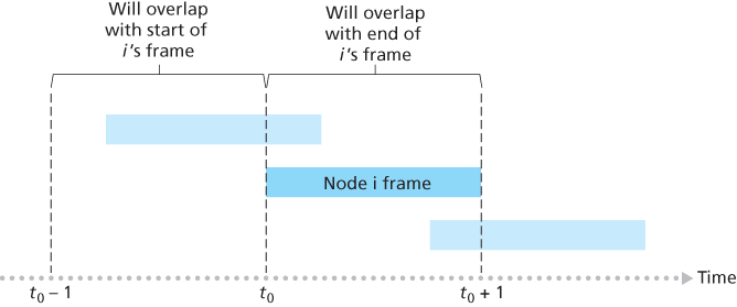
To determine the maximum efficiency of pure ALOHA, we focus on an individual node. We’ll make the same assumptions as in our slotted ALOHA analysis and take the frame transmission time to be the unit of time. At any given time, the probability that a node is transmitting a frame is p. Suppose this frame begins transmission at time . In order for this frame to be successfully transmitted, no other nodes can begin their transmission in the interval of time . Such a transmission would overlap with the beginning of the transmission of node _i_’s frame. The probability that all other nodes do not begin a transmission in this interval is . Similarly, no other node can begin a transmission while node i is transmitting, as such a transmission would overlap with the latter part of node _i_’s transmission. The probability that all other nodes do not begin a transmission in this interval is also . Thus, the probability that a given node has a successful transmission is . By taking limits as in the slotted ALOHA case, we find that the maximum efficiency of the pure ALOHA protocol is only —exactly half that of slotted ALOHA. This then is the price to be paid for a fully decentralized ALOHA protocol

Carrier Sense Multiple Access (CSMA)

There are two important rules for polite human conversation:

• Listen before speaking. If someone else is speaking, wait until they are finished. In the networking world, this is called carrier sensing—a node listens to the channel before transmitting. If a frame from another node is currently being transmitted into the channel, a node then waits until it detects no transmissions for a short amount of time and then begins transmission.
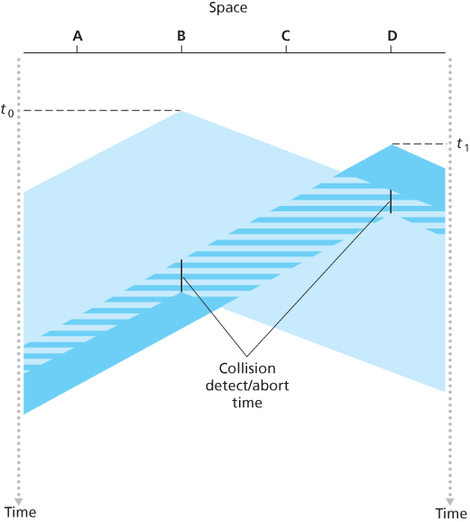
• If someone else begins talking at the same time, stop talking. In the networking world, this is called collision detection—a transmitting node listens to the channel while it is transmitting. If it detects that another node is transmitting an interfering frame, it stops transmitting and waits a random amount of time before repeating the sense-and-transmit-when-idle cycle.

These two rules are embodied in the family of carrier sense multiple access (CSMA) and CSMA with collision detection (CSMA/CD) protocols [Kleinrock 1975b; Metcalfe 1976; Lam 1980; Rom 1990].

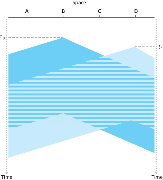
It is evident that the end-to-end channel propagation delay of a broadcast channel—the time it takes for a signal to propagate from one of the nodes to another—will play a crucial role in determining its performance. The longer this propagation delay, the larger the chance that a carrier-sensing node is not yet able to sense a transmission that has already begun at another node in the network.

Carrier Sense Multiple Access with Collision Dection (CSMA/CD)

Ading collision detection to a multiple access protocol will help protocol performance by not transmitting a useless, damaged (by interference with a frame from another node) frame in its entirety.

The need to wait a random (rather than fixed) amount of time is hopefully clear—if two nodes transmitted frames at the same time and then both waited the same fixed amount of time, they’d continue colliding forever. But what is a good interval of time from which to choose the random backoff time? What we’d like is an interval that is short when the number of colliding nodes is small, and long when the number of colliding nodes is large.

The binary exponential backoff algorithm, used in Ethernet as well as in DOCSIS cable network multiple access protocols [DOCSIS 2011], elegantly solves this problem. Specifically, when transmitting a frame that has already experienced n collisions, a node chooses the value of K at random from . Thus, the more collisions experienced by a frame, the larger the interval from which K is chosen. For Ethernet, the actual amount of time a node waits is bit times (i.e., K times the amount of time needed to send 512 bits into the Ethernet) and the maximum value that n can take is capped at 10.

Suppose that a node attempts to transmit a frame for the first time and while transmitting it detects a collision. The node then chooses with probability 0.5 or chooses with probability 0.5. If the node chooses , then it immediately begins sensing the channel. If the node chooses , it waits 512 bit times (e.g., 5.12 microseconds for a 100 Mbps Ethernet) before beginning the sense-and-transmit-when-idle cycle. After a second collision, K is chosen with equal probability from {0,1,2,3}. After three collisions, K is chosen with equal probability from {0,1,2,3,4,5,6,7}.

6.3.3 Taking-Turns Protocols

As with random access protocols, there are dozens of taking-turns protocols, and each one of these protocols has many variations. We’ll discuss two of the more important protocols here. The first one is the polling protocol. The polling protocol requires one of the nodes to be designated as a master node. The master node polls each of the nodes in a round-robin fashion. In particular, the master node first sends a message to node 1, saying that it (node 1) can transmit up to some maximum number of frames. After node 1 transmits some frames, the master node tells node 2 it (node 2) can transmit up to the maximum number of frames. (The master node can determine when a node has finished sending its frames by observing the lack of a signal on the channel.) The procedure continues in this manner, with the master node polling each of the nodes in a cyclic manner.

The second taking-turns protocol is the token-passing protocol. In this protocol there is no master node. A small, special-purpose frame known as a token is exchanged among the nodes in some fixed order. For example, node 1 might always send the token to node 2, node 2 might always send the token to node 3, and node N might always send the token to node 1. When a node receives a token, it holds onto the token only if it has some frames to transmit; otherwise, it immediately forwards the token to the next node. If a node does have frames to transmit when it receives the token, it sends up to a maximum number of frames and then forwards the token to the next node.

6.4 Switched Local Area Networks

6.4.1 Link-Layer Addressing and ARP

MAC Addresses

In truth, it is not hosts and routers that have link-layer addresses but rather their adapters (that is, network interfaces) that have link-layer addresses. A host or router with multiple network interfaces will thus have multiple link-layer addresses associated with it, just as it would also have multiple IP addresses associated with it. It’s important to note, however, that link-layer switches do not have link-layer addresses associated with their interfaces that connect to hosts and routers. This is because the job of the link-layer switch is to carry datagrams between hosts and routers; a switch does this job transparently, that is, without the host or router having to explicitly address the frame to the intervening switch. A link-layer address is variously called a LAN address, a physical address, or a MAC address. For most LANs (including Ethernet and 802.11 wireless LANs), the MAC address is 6 bytes long, giving possible MAC addresses. These 6-byte addresses are typically expressed in hexadecimal notation, with each byte of the address expressed as a pair of hexadecimal numbers. Although MAC addresses were designed to be permanent, it is now possible to change an adapter’s MAC address via software.

The IEEE manages the MAC address space. In particular, when a company wants to manufacture adapters, it purchases a chunk of the address space consisting of addresses for a nominal fee. IEEE allocates the chunk of addresses by fixing the first 24 bits of a MAC address and letting the company create unique combinations of the last 24 bits for each adapter.

An adapter’s MAC address has a flat structure (as opposed to a hierarchical structure) and doesn’t change no matter where the adapter goes. In contrast, IP addresses have a hierarchical structure (that is, a network part and a host part), and a host’s IP addresses needs to be changed when the host moves.

When an adapter wants to send a frame to some destination adapter, the sending adapter inserts the destination adapter’s MAC address into the frame and then sends the frame into the LAN. As we will soon see, a switch occasionally broadcasts an incoming frame onto all of its interfaces. Thus, an adapter may receive a frame that isn’t addressed to it. Thus, when an adapter receives a frame, it will check to see whether the destination MAC address in the frame matches its own MAC address. If there is a match, the adapter extracts the enclosed datagram and passes the datagram up the protocol stack. If there isn’t a match, the adapter discards the frame, without passing the network-layer datagram up. Thus, the destination only will be interrupted when the frame is received.

However, sometimes a sending adapter does want all the other adapters on the LAN to receive and process the frame it is about to send. In this case, the sending adapter inserts a special MAC broadcast address into the destination address field of the frame. For LANs that use 6-byte addresses (such as Ethernet and 802.11), the broadcast address is a string of 48 consecutive 1s (that is, FF-FF-FF-FF-FF-FF in hexadecimal notation).

Address Resolution Protocol (ARP)

Because there are both network-layer addresses (for example, Internet IP addresses) and link-layer addresses (that is, MAC addresses), there is a need to translate between them. For the Internet, this is the job of the Address Resolution Protocol (ARP) [RFC 826].

ARP resolves IP addresses only for hosts and router interfaces on the same subnet.

Each host and router has an ARP table in its memory, which contains mappings of IP addresses to MAC addresses. The ARP table also contains a time-to-live (TTL) value, which indicates when each mapping will be deleted from the table. Note that a table does not necessarily contain an entry for every host and router on the subnet; some may have never been entered into the table, and others may have expired. A typical expiration time for an entry is 20 minutes from when an entry is placed in an ARP table.

Suppose 222.222.222.220 wants to send a datagram to 222.222.222.222. In this case, the sender uses the ARP protocol to resolve the address. First, the sender constructs a special packet called an ARP packet. An ARP packet has several fields, including the sending and receiving IP and MAC addresses. Both ARP query and response packets have the same format. The purpose of the ARP query packet is to query all the other hosts and routers on the subnet to determine the MAC address corresponding to the IP address that is being resolved.

222.222.222.220 passes an ARP query packet to the adapter along with an indication that the adapter should send the packet to the MAC broadcast address, namely, FF-FF-FF-FF-FF-FF. The adapter encapsulates the ARP packet in a link-layer frame, uses the broadcast address for the frame’s destination address, and transmits the frame into the subnet. Recalling our social security number/postal address analogy, an ARP query is equivalent to a person shouting out in a crowded room of cubicles in some company. The frame containing the ARP query is received by all the other adapters on the subnet, and (because of the broadcast address) each adapter passes the ARP packet within the frame up to its ARP module. Each of these ARP modules checks to see if its IP address matches the destination IP address in the ARP packet. The one with a match sends back to the querying host a response ARP packet with the desired mapping. The querying host 222.222.222.220 can then update its ARP table and send its IP datagram, encapsulated in a link-layer frame whose destination MAC is that of the host or router responding to the earlier ARP query.

However, an ARP packet has fields containing link-layer addresses and thus is arguably a link-layer protocol, but it also contains network-layer addresses and thus is also arguably a network-layer protocol.

Sending a Datagram off the Subnet

For each router interface there is also an ARP module (in the router) and an adapter. Because the router has two interfaces, it has two IP addresses, two ARP modules, and two adapters. Of course, each adapter in the network has its own MAC address.

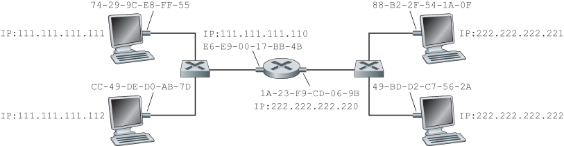
Specifically, suppose that host 111.111.111.111 wants to send an IP datagram to a host 222.222.222.222. The sending host passes the datagram to its adapter, as usual. But the sending host must also indicate to its adapter an appropriate destination MAC address. If the sending adapter were to use that MAC address, then none of the adapters on Subnet 1 would bother to pass the IP datagram up to its network layer, since the frame’s destination address would not match the MAC address of any adapter on Subnet 1. The datagram would just die and go to datagram heaven.

In order for a datagram to go from 111.111.111.111 to a host on Subnet 2, the datagram must first be sent to the router interface 111.111.111.110, which is the IP address of the first-hop router on the path to the final destination. Thus, the appropriate MAC address for the frame is the address of the adapter for router interface 111.111.111.110, namely, E6-E9-00-17-BB-4B. How does the sending host acquire the MAC address for 111.111.111.110? By using ARP, of course! Once the sending adapter has this MAC address, it creates a frame (containing the datagram addressed to 222.222.222.222) and sends the frame into Subnet 1. The router adapter on Subnet 1 sees that the link-layer frame is addressed to it, and therefore passes the frame to the network layer of the router. Hooray—the IP datagram has successfully been moved from source host to the router! But we are not finished. We still have to move the datagram from the router to the destination. The router now has to determine the correct interface on which the datagram is to be forwarded. This is done by consulting a forwarding table in the router. The forwarding table tells the router that the datagram is to be forwarded via router interface 222.222.222.220. This interface then passes the datagram to its adapter, which encapsulates the datagram in a new frame and sends the frame into Subnet 2. This time, the destination MAC address of the frame is indeed the MAC address of the ultimate destination. And how does the router obtain this destination MAC address? From ARP, of course!

6.4.2 Ethernet

Ethernet Frame Structure

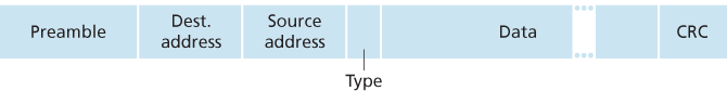
Let’s now examine the six fields of the Ethernet frame:

• Data field (46 to 1,500 bytes). This field carries the IP datagram. The maximum transmission unit (MTU) of Ethernet is 1,500 bytes. This means that if the IP datagram exceeds 1,500 bytes, then the host has to fragment the datagram. The minimum size of the data field is 46 bytes. This means that if the IP datagram is less than 46 bytes, the data field has to be “stuffed” to fill it out to 46 bytes. When stuffing is used, the data passed to the network layer contains the stuffing as well as an IP datagram. The network layer uses the length field in the IP datagram header to remove the stuffing.
• Destination address (6 bytes).
• Source address (6 bytes).
• Type field (2 bytes). The type field permits Ethernet to multiplex network-layer protocols. To understand this, we need to keep in mind that hosts can use other network-layer protocols besides IP. In fact, a given host may support multiple network-layer protocols using different protocols for different applications. For this reason, when the Ethernet frame arrives at adapter B, adapter B needs to know to which network-layer protocol it should pass (that is, demultiplex) the contents of the data field. IP and other network-layer protocols (for example, Novell IPX or AppleTalk) each have their own, standardized type number. Furthermore, the ARP protocol (discussed in the previous section) has its own type number, and if the arriving frame contains an ARP packet (i.e., has a type field of 0806 hexadecimal), the ARP packet will be demultiplexed up to the ARP protocol.
• Cyclic redundancy check (CRC) (4 bytes).
• Preamble (8 bytes). The Ethernet frame begins with an 8-byte preamble field. Each of the first 7 bytes of the preamble has a value of 10101010; the last byte is 10101011. The first 7 bytes of the preamble serve to “wake up” the receiving adapters and to synchronize their clocks to that of the sender’s clock.

All of the Ethernet technologies provide connectionless service to the network layer.

Ethernet technologies provide an unreliable service to the network layer. Specifically, when adapter B receives a frame from adapter A, it runs the frame through a CRC check, but neither sends an acknowledgment when a frame passes the CRC check nor sends a negative acknowledgment when a frame fails the CRC check. When a frame fails the CRC check, adapter B simply discards the frame. Thus, adapter A has no idea whether its transmitted frame reached adapter B and passed the CRC check.

Ethernet Technologies

Ethernet comes in many different flavors, with somewhat bewildering acronyms such as 10BASE-T, 10BASE-2, 100BASE-T, 1000BASE-LX, 10GBASE-T and 40GBASE-T. These and many other Ethernet technologies have been standardized over the years by the IEEE 802.3 CSMA/CD (Ethernet) working group [IEEE 802.3 2012]. While these acronyms may appear bewildering, there is actually considerable order here. The first part of the acronym refers to the speed of the standard: 10, 100, 1000, or 10G, for 10 Megabit (per second), 100 Megabit, Gigabit, 10 Gigabit and 40 Gigibit Ethernet, respectively. “BASE” refers to baseband Ethernet, meaning that the physical media only carries Ethernet traffic; almost all of the 802.3 standards are for baseband Ethernet. The final part of the acronym refers to the physical media itself; Ethernet is both a link-layer and a physical-layer specification and is carried over a variety of physical media including coaxial cable, copper wire, and fiber. Generally, a “T” refers to twisted-pair copper wires.

In the days of bus topologies and hub-based star topologies, Ethernet was clearly a broadcast link in which frame collisions occurred when nodes transmitted at the same time. To deal with these collisions, the Ethernet standard included the CSMA/CD protocol, which is particularly effective for a wired broadcast LAN spanning a small geographical region. But if the prevalent use of Ethernet today is a switch-based star topology, using store-and-forward packet switching, is there really a need anymore for an Ethernet MAC protocol? As we’ll see shortly, a switch coordinates its transmissions and never forwards more than one frame onto the same interface at any time. Furthermore, modern switches are full-duplex, so that a switch and a node can each send frames to each other at the same time without interference. In other words, in a switch-based Ethernet LAN there are no collisions and, therefore, there is no need for a MAC protocol!

6.4.3 Link-Layer Switches

Forwarding and Filtering

Filtering is the switch function that determines whether a frame should be forwarded to some interface or should just be dropped. Forwarding is the switch function that determines the interfaces to which a frame should be directed, and then moves the frame to those interfaces. Switch filtering and forwarding are done with a switch table. The switch table contains entries for some, but not necessarily all, of the hosts and routers on a LAN. An entry in the switch table contains (1) a MAC address, (2) the switch interface that leads toward that MAC address, and (3) the time at which the entry was placed in the table.

To understand how switch filtering and forwarding work, suppose a frame with destination address DD-DD-DD-DD-DD-DD arrives at the switch on interface x. The switch indexes its table with the MAC address DD-DD-DD-DD-DD-DD. There are three possible cases:

• There is no entry in the table for DD-DD-DD-DD-DD-DD. In this case, the switch forwards copies of the frame to the output buffers preceding all interfaces except for interface x. In other words, if there is no entry for the destination address, the switch broadcasts the frame.
• There is an entry in the table, associating DD-DD-DD-DD-DD-DD with interface x. In this case, the frame is coming from a LAN segment that contains adapter DD-DD-DD-DD-DD-DD. There being no need to forward the frame to any of the other interfaces, the switch performs the filtering function by discarding the frame.
• There is an entry in the table, associating DD-DD-DD-DD-DD-DD with interface  In this case, the frame needs to be forwarded to the LAN segment attached to interface y. The switch performs its forwarding function by putting the frame in an output buffer that precedes interface y.

Self-Learning

A switch has the wonderful property (particularly for the already-overworked network administrator) that its table is built automatically, dynamically, and autonomously—without any intervention from a network administrator or from a configuration protocol. In other words, switches are self-learning. This capability is accomplished as follows:

1. The switch table is initially empty.
2. For each incoming frame received on an interface, the switch stores in its table (1) the MAC address in the frame’s source address field, (2) the interface from which the frame arrived, and (3) the current time. In this manner the switch records in its table the LAN segment on which the sender resides. If every host in the LAN eventually sends a frame, then every host will eventually get recorded in the table.
3. The switch deletes an address in the table if no frames are received with that address as the source address after some period of time (the aging time).

Switches Versus Routers

	Hubs	Routers	Switches
Traffic isolation	No	Yes	Yes
Plug and play	Yes	No	Yes
Optimal routing	No	Yes	No

6.4.4 Virtual Local Area Networks (VLANs)

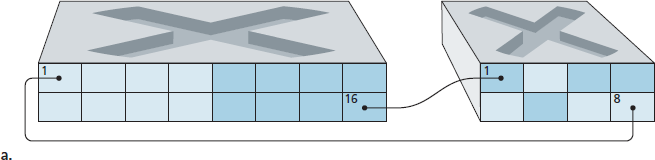
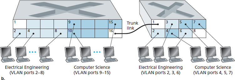
A switch that supports VLANs allows multiple virtual local area networks to be defined over a single physical local area network infrastructure. Hosts within a VLAN communicate with each other as if they (and no other hosts) were connected to the switch.

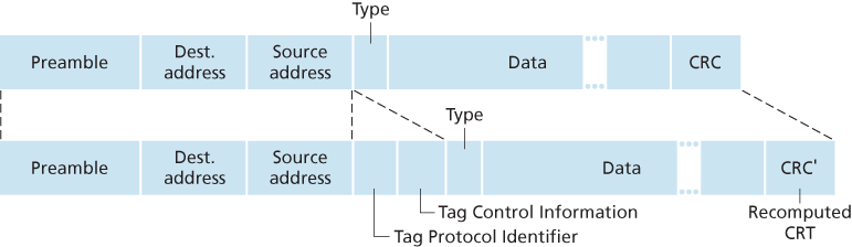
In the VLAN trunking approach, a special port on each switch (port 16 on the left switch and port 1 on the right switch) is configured as a trunk port to interconnect the two VLAN switches. The trunk port belongs to all VLANs, and frames sent to any VLAN are forwarded over the trunk link to the other switch. But this raises yet another question: How does a switch know that a frame arriving on a trunk port belongs to a particular VLAN? The IEEE has defined an extended Ethernet frame format, 802.1Q, for frames crossing a VLAN trunk. The 802.1Q frame consists of the standard Ethernet frame with a four-byte VLAN tag added into the header that carries the identity of the VLAN to which the frame belongs. The VLAN tag is added into a frame by the switch at the sending side of a VLAN trunk, parsed, and removed by the switch at the receiving side of the trunk. The VLAN tag itself consists of a 2-byte Tag Protocol Identifier (TPID) field (with a fixed hexadecimal value of 81-00), a 2-byte Tag Control Information field that contains a 12-bit VLAN identifier field, and a 3-bit priority field that is similar in intent to the IP datagram TOS field.

6.5 Link Virtualization: A Network as a Link Layer

Unlike the circuit-switched telephone network, MPLS is a packet-switched, virtual-circuit network in its own right. It has its own packet formats and forwarding behaviors.

6.5.1 Multiprotocol Label Switching (MPLS)

Multiprotocol Label Switching (MPLS) evolved from a number of industry efforts in the mid-to-late 1990s to improve the forwarding speed of IP routers by adopting a key concept from the world of virtual-circuit networks: a fixed-length label. The goal was not to abandon the destination-based IP datagram-forwarding infrastructure for one based on fixed-length labels and virtual circuits, but to augment it by selectively labeling datagrams and allowing routers to forward datagrams based on fixed-length labels (rather than destination IP addresses) when possible. Importantly, these techniques work hand-in-hand with IP, using IP addressing and routing. The IETF unified these efforts in the MPLS protocol [RFC 3031, RFC 3032], effectively blending VC techniques into a routed datagram network.

A link-layer frame transmitted between MPLS-capable devices has a small MPLS header added between the layer-2 (e.g., Ethernet) header and layer-3 (i.e., IP) header. RFC 3032 defines the format of the MPLS header for such links; headers are defined for ATM and frame-relayed networks as well in other RFCs.

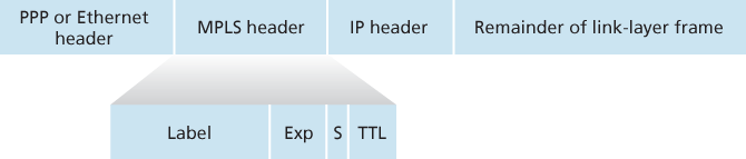
An MPLS-enhanced frame can only be sent between routers that are both MPLS capable (since a non-MPLS-capable router would be quite confused when it found an MPLS header where it had expected to find the IP header!). An MPLS-capable router is often referred to as a label-switched router, since it forwards an MPLS frame by looking up the MPLS label in its forwarding table and then immediately passing the datagram to the appropriate output interface. Thus, the MPLS-capable router need not extract the destination IP address and perform a lookup of the longest prefix match in the forwarding table.

We note that MPLS can, and has, been used to implement so-called virtual private networks (VPNs). In implementing a VPN for a customer, an ISP uses its MPLS-enabled network to connect together the customer’s various networks. MPLS can be used to isolate both the resources and addressing used by the customer’s VPN from that of other users crossing the ISP’s network; see [DeClercq 2002] for details.

6.6 Data Center Networking

A load balancer is sometimes referred to as a “layer-4 switch” since it makes decisions based on the destination port number (layer 4) as well as destination IP address in the packet.