Chapter 9 Graph Algorithms

9.1 Definitions

A graph consists of a set of vertices, , and a set of edges, . Each edge is a pair , where . Edges are sometimes referred to as arcs. If the pair is ordered, then the graph is directed. Directed graphs are sometimes referred to as digraphs. Vertex is adjacent to if and only if . In an undirected graph with edge , and hence , is adjacent to and is adjacent to . Sometimes an edge has a third component, known as either a weight or a cost.

A path in a graph is a sequence of vertices such that for . The length of such a path is the number of edges on the path, which is equal to . We allow a path from a vertex to itself; if this path contains no edges, then the path length is . This is a convenient way to define an otherwise special case. If the graph contains an edge from a vertex to itself, then the path is sometimes referred to as a loop. The graphs we will consider will generally be loopless. A simple path is a path such that all vertices are distinct, except that the first and last could be the same.

A cycle in a directed graph is a path of length at least such that ; this cycle is simple if the path is simple. For undirected graphs, we require that the edges be distinct. The logic of these requirements is that the path , in an undirected graph should not be considered a cycle, because and are the same edge. A directed graph is acyclic if it has no cycles. A directed acyclic graph is sometimes referred to by its abbreviation, DAG.

An undirected graph is connected if there is a path from every vertex to every other vertex. A directed graph with this property is called strongly connected. If a directed graph is not strongly connected, but the underlying graph (without direction to the arcs) is connected, then the graph is said to be weakly connected. A complete graph is a graph in which there is an edge between every pair of vertices.

9.1.1 Representation of Graphs

One simple way to represent a graph is to use a two-dimensional array. This is known as an adjacency matrix representation. For each edge , we set A[u][v] to true.

Although this has the merit of extreme simplicity, the space requirement is , which can be prohibitive if the graph does not have very many edges. An adjacency matrix is an appropriate representation if the graph is dense: .

If the graph is not dense, in other words, if the graph is sparse, a better solution is an adjacency list representation. For each vertex, we keep a list of all adjacent vertices. The space requirement is then .

9.2 Topological Sort

A topological sort is an ordering of vertices in a directed acyclic graph, such that if there is a path from to , then appears after in the ordering.

It is clear that a topological ordering is not possible if the graph has a cycle. Furthermore, the ordering is not necessarily unique; any legal ordering will do. In the graph, and are both topological orderings.

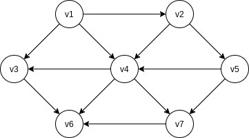
A simple algorithm to find a topological ordering is first to find any vertex with no incoming edges. We can then print this vertex, and remove it, along with its edges, from the graph. Then we apply this same strategy to the rest of the graph.

To formalize this, we define the indegree of a vertex as the number of edges .

Vertex	1	2	3	4	5	6	7
	0	0	0	0	0	0	0
	1	0	0	0	0	0	0
	2	1	1	1	0	0	0
	3	2	1	0	0	0	0
	1	1	0	0	0	0	0
	3	3	3	3	2	1	0
	2	2	2	1	0	0	0
Enqueue
Dequeue

void topsort() throws CycleFoundException {
    Queue<Vertex> q = new Queue<Vertex>();
    int counter = 0;
    
    for (Vertex v: vertexList)
        if (v.indegree == 0)
            q.enqueue(v);
    
    while (!q.isEmpty()) {
        Vertex v = q.dequeue();
        v.topNum = ++counter;
        
        for (Vertex w: v.getAdjacentVertexList())
            if (if --w.indegree == 0)
                q.enqueue(w);
    }
    
    if (counter != NUM_VERTICES)
        throw new CycleFoundException();
}

We can remove this inefficiency by keeping all the (unassigned) vertices of indegree in a special box. To implement the box, we can use either a stack or a queue; we will use a queue. First, the indegree is computed for every vertex. Then all vertices of indegree are placed on an initially empty queue. While the queue is not empty, a vertex is removed, and all vertices adjacent to have their indegrees decremented. A vertex is put on the queue as soon as its indegree falls to . The topological ordering then is the order in which the vertices dequeue.

9.3 Shortest-Path Algorithms

The input is a weighted graph: associated with each edge is a cost to traverse the edge. The cost of a path is $\sum^{N-1}{i=1}c{i,i+1}$. This is referred to as the weighted path length. The unweighted path length is merely the number of edges on the path, namely, .

---

Single-Source Shortest-Path Problem.

Given as input a weighted graph, , and a distinguished vertex, , find the shortest weighted path from to every other vertex in .

---

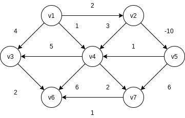
This loop is known as a negative-cost cycle; when one is present in the graph, the shortest paths are not defined.

9.3.1 Unweighted Shortest Paths

Using some vertex, , which is an input parameter, we would like to find the shortest path from to all other vertices. Suppose we choose to be . Immediately, we can tell that the shortest path from to is then a path of length .

This strategy for searching a graph is known as breadth-first search. It operates by processing vertices in layers: The vertices closest to the start are evaluated first, and the most distant vertices are evaluated last. This is much the same as a level-order traversal for trees.

For each vertex, we will keep track of three pieces of information. First, we will keep its distance from in the entry . Initially all vertices are unreachable except for , whose path length is . The entry in is the bookkeeping variable, which will allow us to print the actual paths. The entry known is set to true after a vertex is processed. Initially, all entries are not known, including the start vertex. When a vertex is marked known, we have a guarantee that no cheaper path will ever be found, and so processing for that vertex is essentially complete.

v	known
	F		0
	F		0
	F	0	0
	F		0
	F		0
	F		0
	F		0

void unweighted(Vertex s) {
    for (Vertex v: vertexList) {
        v.dist = INFINITY;
        v.known = false;
    }
    
    s.dist = 0;
    
    for (int currDist = 0; currDist < NUM_VERTICES; currDist++)
        for (Vertex v: VertexList)
            if (!v.known && v.dist == currDist) {
                v.known = true;
                for (Vertex w: v.getAdjacentVertexList())
                    if (w.dist == INFINITY) {
                        w.dist = currDist + 1;
                        w.path = v;
                    }
            }
}

The running time of the algorithm is , because of the doubly nested for loops. An obvious inefficiency is that the outside loop continues until NUM_VERTICES - 1, even if all the vertices become known much earlier.

We can remove the inefficiency in much the same way as was done for topological sort.

void unweighted(Vertex s) {
    Queue<Vertex> q = new Queue<Vertex>();
    
    for (Vertex v: vertexList)
        v.dist = INFINITY;
    
    s.dist = 0;
    q.enqueue(s);
    
    while (!q.isEmpty()) {
        Vertex v = q.dequeue();
        
        for (Vertex w: v.getAdjacentVertexList())
            if (w.dist == INFINITY) {
                w.dist = v.dist + 1;
                w.path = v;
                q.enqueue(w);
            }
    }
}

9.3.2 Dijkstra’s Algorithm

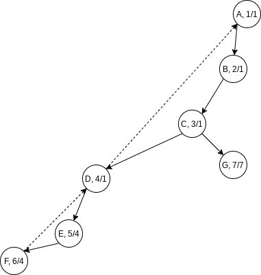
The general method to solve the single-source shortest-path problem is known as Dijkstra’s algorithm. This thirty-year-old solution is a prime example of a greedy algorithm. Greedy algorithms generally solve a problem in stages by doing what appears to be the best thing at each stage.

In the unweighted case, we set if . Thus, we essentially lowered the value of if vertex offered a shorter path. If we apply the same logic to the weighted case, then we should set if this new value for would be an improvement.

1. Initial configuration of table used in Dijkstra’s algorithm

   v	known
   	F	0	0
   	F		0
   	F		0
   	F		0
   	F		0
   	F		0
   	F		0

2. After is declared known

   v	known
   	T	0	0
   	F	2
   	F		0
   	F	1
   	F		0
   	F		0
   	F		0

3. After is declared known

   v	known
   	T	0	0
   	F	2
   	F	3
   	T	1
   	F	3
   	F	9
   	F	5

4. After is declared known

   v	known
   	T	0	0
   	T	2
   	F	3
   	T	1
   	F	3
   	F	9
   	F	5

5. After and then are declared known

   v	known
   	T	0	0
   	T	2
   	T	3
   	T	1
   	T	3
   	F	8
   	F	5

6. After is declared known

   v	known
   	T	0	0
   	T	2
   	T	3
   	T	1
   	T	3
   	F	6
   	T	5

7. After is declared known and algorithm terminates

   v	known
   	T	0	0
   	T	2
   	T	3
   	T	1
   	T	3
   	T	6
   	T	5

class Vertex {
    public List adj;
    public boolean known;
    public DistType dist;
    public Vertex path;
}

public class Main() {
    void printPath(Vertex v) {
        if (v.path != null ) {
            printPath(v.path);
            System.out.print(" to ");
        }
        System.out.print(v);
    }
    
    void dijkstra(Vertex s) {
        for (Vertex v: vertexList) {
            v.dist = INFINITY;
            v.known = false;
        }
        
        s.dist = 0;
        
        while (vertexList.hasUnknownVertex()) {
            Vertex v = vertexList.getSmallestUnknownDistanceVertex();
            
            v.known = true;
            
            for (Vertex w: v.getAdjacentVertexList())
                if (!w.known) {
                    DistType cvw = cost(v, w);
                    
                    if (v.dist + cvw < w.dist) {
                        w.dist = v.dist + cvw;
                        w.path = v;
                    }
                }
        }
    }
}

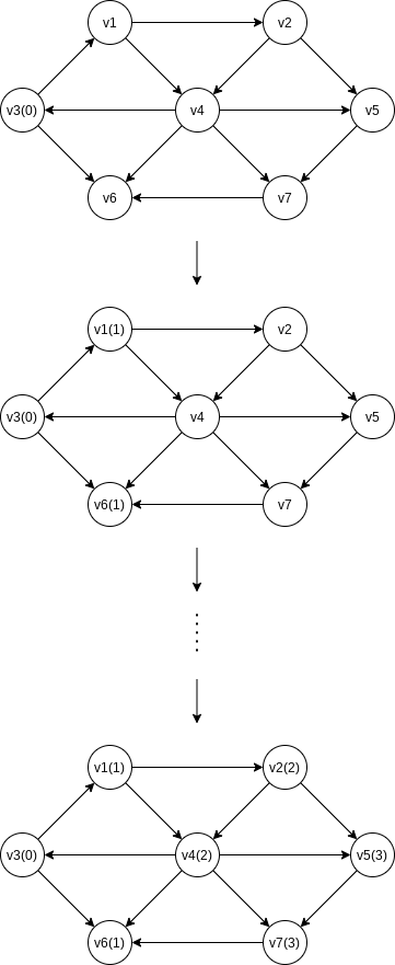
9.3.4 Acyclic Graphs

If the graph is known to be acyclic, we can improve Dijkstra’s algorithm by changing the order in which vertices are declared known, otherwise known as the vertex selection rule. The new rule is to select vertices in topological order.

This selection rule works because when a vertex is selected, its distance, , can no longer be lowered, since by the topological ordering rule it has no incoming edges emanating from unknown nodes.

There is no need for a priority queue with this selection rule; the running time is , since the selection takes constant time.

A more important use of acyclic graphs is critical path analysis. Each node represents an activity that must be performed, along with the time it takes to complete the activity. This graph is thus known as an activity-node graph.

To perform these calculations, we convert the activity-node graph to an event-node graph. Each event corresponds to the completion of an activity and all its dependent activities.

To find the earliest completion time of the project, we merely need to find the length of the longest path from the first event to the last event. For general graphs, the longest-path problem generally does not make sense, because of the possibility of positive-cost cycles. These are the equivalent of negative-cost cycles in shortest-path problems.

9.4 Network Flow Problems

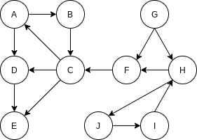
Suppose we are given a directed graph with edge capacities . These capacities could represent the amount of water that could flow through a pipe or the amount of traffic that could flow on a street between two intersections. We have two vertices: , which we call the source, and , which is the sink. Through any edge, , at most units of “flow” may pass. At any vertex, , that is not either or , the total flow coming in must equal the total flow going out. The maximum flow problem is to determine the maximum amount of flow that can pass from to .

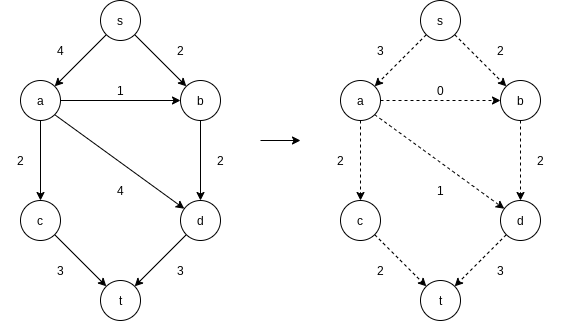
9.4.1 A Simple Maximum-Flow Algorithm

A first attempt to solve the problem proceeds in stages. We start with our graph, , and construct a flow graph . tells the flow that has been attained at any stage in the algorithm. Initially all edges in have no flow, and we hope that when the algorithm terminates, contains a maximum flow. We also construct a graph, , called the residual graph. tells, for each edge, how much more flow can be added. We can calculate this by subtracting the current flow from the capacity for each edge. An edge in is known as a residual edge.

At each stage, we find a path in from to . This path is known as an augmenting path.

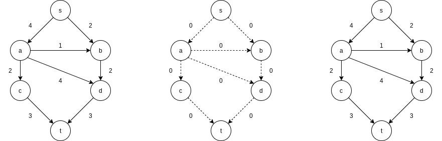
There are many paths from s to t in the residual graph. Suppose we select . Then we can send two units of flow through every edge on this path. We will adopt the convention that once we have filled (saturated) an edge, it is removed from the residual graph.

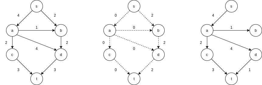
Next, we might select the path which also allows two units of flow.

The only path left to select is , which allows one unit of flow.

The algorithm terminates at this point, because is unreachable from . The resulting flow of happens to be the maximum. To see what the problem is, suppose that with our initial graph, we chose the path . This path allows three units of flow and thus seems to be a good choice. The result of this choice, however, leaves only one path from to in the residual graph; it allows one more unit of flow, and thus, our algorithm has failed to find an optimal solution. This is an example of a greedy algorithm that does not work.

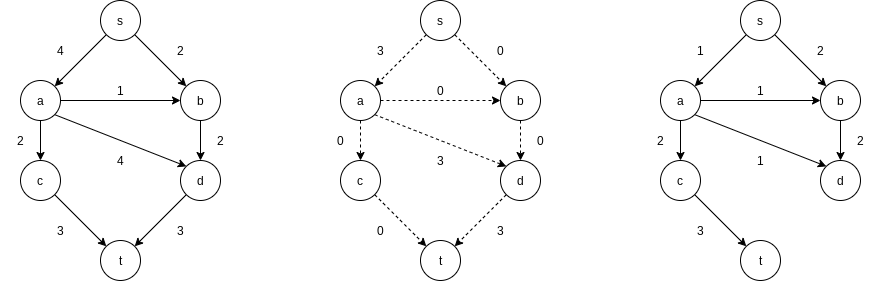
In order to make this algorithm work, we need to allow the algorithm to change its mind. To do this, for every edge with flow in the flow graph, we will add an edge in the residual graph of capacity . In effect, we are allowing the algorithm to undo its decisions by sending flow back in the opposite direction. Starting from our original graph and selecting the augmenting path .

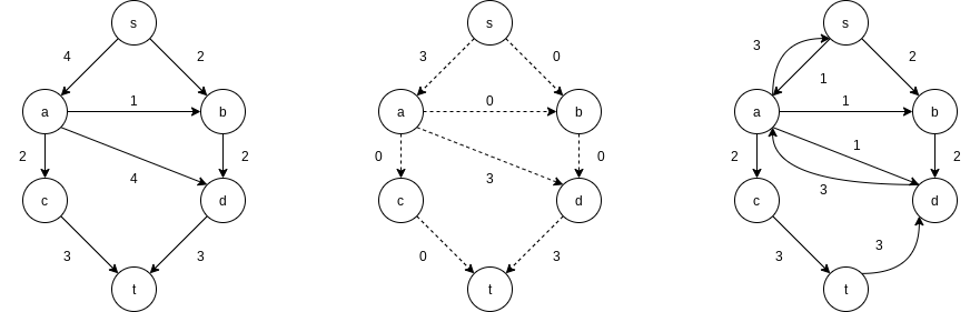
Notice that in the residual graph, there are edges in both directions between and . Either one more unit of flow can be pushed from and , or up to three units can be pushed back – we can undo flow. Now the algorithm finds the augmenting path , of flow . By pushing two units of flow from to , the algorithm takes two units of flow away from the edge and is essentially changing its mind.

A simple method to get around this problem is always to choose the augmenting path that allows the largest increase in flow. Finding such a path is similar to solving a weighted shortest-path problem and a single-line modification to Dijkstra’s algorithm will do the trick. If is the maximum edge capacity, then one can show that augmentations will suffice to find the maximum flow.

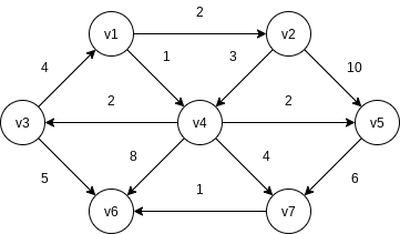
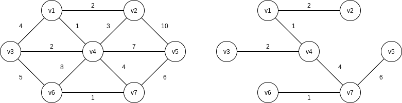
9.5 Minimum Spanning Tree

Informally, a minimum spanning tree of an undirected graph is a tree formed from graph edges that connects all the vertices of at lowest total cost.

9.5.1 Prim’s Algorithm

One way to compute a minimum spanning tree is to grow the tree in successive stages. In each stage, one node is picked as the root, and we add an edge, and thus an associated vertex, to the tree.

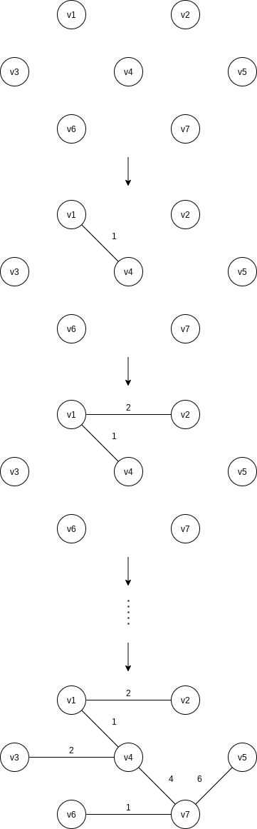
We can see that Prim’s algorithm is essentially identical to Dijkstra’s algorithm for shortest paths. As before, for each vertex we keep values and and an indication of whether it is known or unknown. is the weight of the shortest edge connecting v to a known vertex, and , is the last vertex to cause a change in .

9.5.2 Kruskal’s Algorithm

Formally, Kruskal’s algorithm maintains a forest – a collection of trees. Initially, there are single-node trees. Adding an edge merges two trees into one. When the algorithm terminates, there is only one tree, and this is the minimum spanning tree.

The algorithm terminates when enough edges are accepted. It turns out to be simple to decide whether edge should be accepted or rejected. The appropriate data structure is the union/find algorithm.

Edge	Weight	Action
	1	Accepted
	1	Accepted
	2	Accepted
	2	Accepted
	3	Rejected
	4	Rejected
	4	Accepted
	5	Rejected
	6	Accepted

The invariant we will use is that at any point in the process, two vertices belong to the same set if and only if they are connected in the current spanning forest.

ArrayList<Edge> kruskal(List<Edge> edges, int numVertices) {
    DisjSets ds = new DisjSets(numVertices);
    PriorityQueue<Edge> pq = new PriorityQueue<>(edges);
    List<Edge> mst = new ArrayList<>();
    
    while (mst.size() != numVertices - 1) {
        Edge e = pq.deleteMin();
        SetType uset = ds.find(e.getu());
        SetType vset = ds.find(e.getv());
        
        if (uset != vset) {
            mst.add(e);
            ds.union(uset, vset);
        }
    }
    
    return mst;
}

The worst-case running time of this algorithm is , which is dominated by the heap operations. Notice that since , this running time is actually . In practice, the algorithm is much faster than this time bound would indicate.

9.6 Applications of Depth-First Search

Depth-first search is a generalization of preorder traversal. Starting at some vertex, , we process and then recursively traverse all vertices adjacent to . If this process is performed on a tree, then all tree vertices are systematically visited in a total of time, since . If we perform this process on an arbitrary graph, we need to be careful to avoid cycles.

void dfs(Vertex v) {
    v.visited = true;
    for (Vertex w: v.getAdjacentVertexList())
        if (!w.visited)
            dfs(w);
}

9.6.2 Biconnectivity

A connected undirected graph is biconnected if there are no vertices whose removal disconnects the rest of the graph.

If a graph is not biconnected, the vertices whose removal would disconnect the graph are known as articulation points.

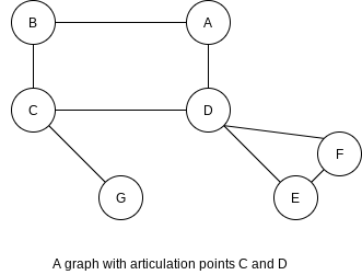
Depth-first search provides a linear-time algorithm to find all articulation points in a connected graph. First, starting at any vertex, we perform a depth-first search and number the nodes as they are visited. For each vertex , we call this preorder number Num(v). Then, for every vertex in the depth-first search spanning tree, we compute the lowest-numbered vertex, which we call Low(v), that is reachable from by taking zero or more tree edges and then possibly one back edge (in that order).

We can efficiently compute Low by performing a postorder traversal of the depth-first spanning tree. By the definition of Low, Low(v) is the minimum of:

1. Num(v)
2. the lowest Num(w) among all back edges
3. the lowest Low(w) among all tree edges

All that is left to do is to use this information to find articulation points. The root is an articulation point if and only if it has more than one child. Any other vertex is an articulation point if and only if has some child such that .

void assignNum(Vertex v) {
    v.num = counter++;
    v.visited = true;
    for (Vertex w: v.getAdjacentVertexList())
        if (!w.visited) {
            w.parent = v;
            assignNum(w);
        }
}

void assignLow(Vertex v) {
    v.low = v.num;
    for (Vertex w: v.getAdjacentVertexList()) {
        if (w.num > v.num) {
            assignLow(w);
            if (w.low >= v.num)
                System.out.println(v + " is an articulation point");
            v.low = min(v.low, w.low);
        } else if (v.parent != w)
            v.low = min(v.low, w.num);
    }
}

9.6.4 Directed Graphs

Using the same strategy as with undirected graphs, directed graphs can be traversed in linear time, using depth-first search. If the graph is not strongly connected, a depth-first search starting at some node might not visit all nodes.

We arbitrarily start the depth-first search at vertex . This visits vertices and . We then restart at some unvisited vertex. Arbitrarily, we start at , which visits and . Finally, we start at , which is the last vertex that needs to be visited.

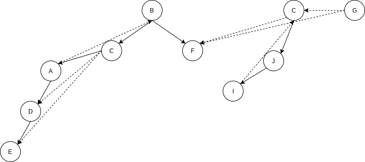
9.6.5 Finding Strong Components

By performing two depth-first searches, we can test whether a directed graph is strongly connected, and if it is not, we can actually produce the subsets of vertices that are strongly connected to themselves.

First, a depth-first search is performed on the input graph . The vertices of are numbered by a postorder traversal of the depth-first spanning forest, and then all edges in are reversed, forming .

The algorithm is completed by performing a depth-first search on , always starting a new depth-first search at the highest-numbered vertex.

9.7 Introduction to NP-Completeness

9.7.1 Easy vs. Hard

Just as real numbers are not sufficient to express a solution to , one can prove that computers cannot solve every problem that happens to come along. These “impossible” problems are called undecidable problems.

One particular undecidable problem is the halting problem. Is it possible to have your Java compiler have an extra feature that not only detects syntax errors, but also all infinite loops? This seems like a hard problem, but one might expect that if some very clever programmers spent enough time on it, they could produce this enhancement.

The intuitive reason that this problem is undecidable is that such a program might have a hard time checking itself. For this reason, these problems are sometimes called recursively undecidable.

9.7.2 The Class NP

NP stands for nondeterministic polynomial-time. A deterministic machine, at each point in time, is executing an instruction. Depending on the instruction, it then goes to some next instruction, which is unique. A nondeterministic machine has a choice of next steps. It is free to choose any that it wishes, and if one of these steps leads to a solution, it will always choose the correct one. Furthermore, nondeterminism is not as powerful as one might think. For instance, undecidable problems are still undecidable, even if nondeterminism is allowed.

Notice also that not all decidable problems are in NP. Consider the problem of deter mining whether a graph does not have a Hamiltonian cycle. To prove that a graph has a Hamiltonian cycle is a relatively simple matter – we just need to exhibit one. Nobody knows how to show, in polynomial time, that a graph does not have a Hamiltonian cycle. It seems that one must enumerate all the cycles and check them one by one. Thus the Non-Hamiltonian cycle problem is not known to be in NP.

9.7.3 NP-Complete Problems

An NP-complete problem has the property that any problem in NP can be polynomially reduced to it.

A problem can be reduced to as follows: Provide a mapping so that any instance of can be transformed to an instance of . Solve , and then map the answer back to the original.

---

Traveling Salesman Problem.

Given a complete graph , with edge costs, and an integer , is there a simple cycle that visits all vertices and has total cost ?

---

The traveling salesman problem is NP-complete. It is easy to see that a solution can be checked in polynomial time, so it is certainly in NP. To show that it is NP-complete, we polynomially reduce the Hamiltonian cycle problem to it. To do this we construct a new graph . ‘ has the same vertices as . For , each edge has a weight of if , and otherwise. We choose .

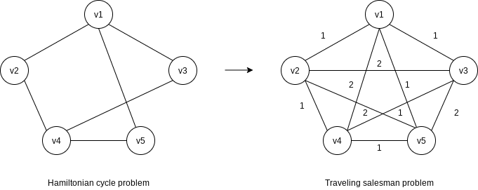
It is easy to verify that has a Hamiltonian cycle if and only if has a traveling salesman tour of total weight .

The first problem that was proven to be NP-complete was the satisfiability problem. The satisfiability problem takes as input a Boolean expression and asks whether the expression has an assignment to the variables that gives a value of true.