Chapter 7 Sorting

7.2 Insertion Sort

7.2.1 The Algorithm

Insertion sort consists of passes. For pass through , insertion sort ensures that the elements in positions through are in sorted order. Insertion sort makes use of the fact that elements in positions through are already known to be in sorted order.

Original	34	8	64	51	32	21	Positions Moved
After p = 1	8	34	64	51	32	21	1
After p = 2	8	34	64	51	32	21	0
After p = 3	8	34	51	64	32	21	1
After p = 4	8	32	34	51	64	21	3
After p = 5	8	21	32	34	51	64	4

public static <AnyType extends Comparable<? super AnyType>> void insertionSort(AnyType[] a) {
    int j;
    for(int p = 1; p < a.length; p++) {
        AnyType tmp = a[p];
        for(j = p; j > 0 && tmp.compareTo(a[j - 1]) < 0; j--)
            a[j] = a[j - 1];
        a[j] = tmp;
    }
}

7.2.2 Analysis of Insertion Sort

Because of the nested loops, each of which can take iterations, insertion sort is . Summing over all gives a total of

If the input is presorted, the running time is , because the test in the inner for loop always fails immediately.

7.3 A Lower Bound for Simple Sorting Algorithms

An inversion in an array of numbers is any ordered pair having the property that but . Notice that this is exactly the number of swaps that needed to be (implicitly) performed by insertion sort. Since there is other work involved in the algorithm, the running time of insertion sort is , where I is the number of inversions in the original array. Thus, insertion sort runs in linear time if the number of inversions is .

We can compute precise bounds on the average running time of insertion sort by computing the average number of inversions in a permutation.

Theorem 7.1.

The average number of inversions in an array of distinct elements is .

Proof.

For any list, , of elements, consider , the list in reverse order. Consider any pair of two elements in the list , with . Clearly, in exactly one of and this ordered pair represents an inversion. The total number of these pairs in a list and its reverse is . Thus, an average list has half this amount, or inversions.

Theorem 7.2.

Any algorithm that sorts by exchanging adjacent elements requires time on average.

Proof.

The average number of inversions is initially . Each swap removes only one inversion, so swaps are required.

7.4 Shellsort

Shellsort works by comparing elements that are distant; the distance between comparisons decreases as the algorithm runs until the last phase, in which adjacent elements are compared. For this reason, Shellsort is sometimes referred to as diminishing increment sort.

Shellsort uses a sequence, , called the increment sequence. Any increment sequence will do as long as , but some choices are better than others. After a phase, using some increment , for every , we have ; all elements spaced apart are sorted. The file is then said to be -sorted.

Original	81	94	11	96	12	35	17	95	28	58	41	75	15
After 5-sort	35	17	11	28	12	41	75	15	96	58	81	94	95
After 3-sort	28	12	11	35	15	41	58	17	94	75	81	96	95
After 1-sort	11	12	15	17	28	35	41	58	75	81	94	95	96

The general strategy to -sort is for each position, , in , place the element in the correct spot among , and so on. Although this does not affect the implementation, a careful examination shows that the action of an -sort is to perform an insertion sort on independent subarrays. This observation will be important when we analyze the running time of Shellsort.

A popular (but poor) choice for increment sequence is to use the sequence suggested by Shell: , and .

public static <AnyType extends Comparable<? super AnyType>> void shellsort(AnyType[] a) {
    int j;
    for(int gap = a.length / 2; gap > 0; gap /= 2)
        for(int i = gap; i < a.length; i++) {
            AnyType tmp = a[i];
            for(j = i; j >= gap && tmp.compareTo(a[j - gap]) < 0; j -= gap)
                a[j] = a[j - gap];
            a[j] = tmp;
        }
}

7.4.1 Worst-Case Analysis of Shellsort

Theorem 7.3.

The worst-case running time of Shellsort, using Shell’s increments, is .

Proof.

The proof requires showing not only an upper bound on the worst-case running time but also showing that there exists some input that actually takes time to run. We prove the lower bound first, by constructing a bad case. First, we choose to be a power of . This makes all the increments even, except for the last increment, which is . Now, we will give as input an array with the largest numbers in the even positions and the smallest numbers in the odd positions (for this proof, the first position is position ). As all the increments except the last are even, when we come to the last pass, the largest numbers are still all in even positions and the smallest numbers are still all in odd positions. The th smallest number () is thus in position before the beginning of the last pass. Restoring the ith element to its correct place requires moving it spaces in the array. Thus, to merely place the smallest elements in the correct place requires at least work.

As we have observed before, a pass with increment consists of insertion sorts of about elements. Since insertion sort is quadratic, the total cost of a pass is . Summing over all passes gives a total bound of . Because the increments form a geometric series with common ratio 2, and the largest term in the series is . Thus we obtain a total bound of .

Theorem 7.4.

The worst-case running time of Shellsort using Hibbard’s increments is .

Proof.

We will prove only the upper bound here.

When we come to -sort the input array, we know that it has already been - and -sorted. Prior to the -sort, consider elements in positions and , . If is a multiple of or , then clearly . We can say more, however. If is expressible as a linear combination (in nonnegative integers) of and , then . As an example, when we come to sort, the file is already and sorted. is expressible as a linear combination of and , because . Thus, cannot be larger than because .

Now, , so and cannot share a common factor. In this case, it is possible to show that all integers that are at least as large as can be expressed as a linear combination of and .

This tells us that the body of the innermost for loop can be executed at most times for each of the positions. This gives a bound of per pass.

Using the fact that about half the increments satisfy , and assuming that is even, the total running time is then

Because both sums are geometric series, and since , this simplifies to

The average-case running time of Shellsort, using Hibbard’s increments, is thought to be , based on simulations, but nobody has been able to prove this. Pratt has shown that the bound applies to a wide range of increment sequences.

Sedgewick has proposed several increment sequences that give an worst-case running time (also achievable). The average running time is conjectured to be for these increment sequences. Empirical studies show that these sequences perform significantly better in practice than Hibbard’s. The best of these is the sequence , in which the terms are either of the form or . This is most easily implemented by placing these values in an array. This increment sequence is the best known in practice, although there is a lingering possibility that some increment sequence might exist that could give a significant improvement in the running time of Shellsort.

7.5 Heapsort

We then perform deleteMin operations. The elements leave the heap smallest first, in sorted order. By recording these elements in a second array and then copying the array back, we sort elements. Since each deleteMin takes time, the total running time is .

Notice that the extra time spent copying the second array back to the first is only , so that this is not likely to affect the running time significantly. The problem is space.

A clever way to avoid using a second array makes use of the fact that after each deleteMin, the heap shrinks by . Thus the cell that was last in the heap can be used to store the element that was just deleted.

private static int leftChild(int i) {
    return 2 * i + 1;
}

private static <AnyType extends Comparable<? super AnyType>> void percDown(AnyType[] a, int i, int n) {
    int child;
    AnyType tmp;
    
    for(tmp = a[i]; leftChild(i) < n; i = child) {
        child = leftChild(i);
        if(child != n - 1 && a[child].compareTo(a[child + 1]) < 0)
            child++;
        if(tmp.compareTo(a[child]) < 0)
            a[i] = a[child];
        else
            break;
    }
    
    a[i] = tmp;
}

public static <AnyType extends Comparable<? super AnyType>> void heapsort(AnyType[] a) {
    for(int i = a.length / 2 - 1; i >= 0; i--)
        percDown(a, i, a.length);
    for(int i = a.length - 1; i > 0; i--) {
        swapReferences(a, 0, i);
        percDown(a, 0, i);
    }
}

7.5.1 Analysis of Heapsort

The first phase, which constitutes the building of the heap, uses less than comparisons. In the second phase, the ith deleteMax uses at most less than comparisons, for a total of at most comparisons (assuming ). Consequently, in the worst case, at most comparisons are used by heapsort.

Experiments have shown that the performance of heapsort is extremely consistent: On average it uses only slightly fewer comparisons than the worst-case bound suggests.

Theorem 7.5.

The average number of comparisons used to heapsort a random permutation of distinct items is .

Proof.

The heap construction phase uses comparisons on average, and so we only need to prove the bound for the second phase. We assume a permutation of .

Suppose the th deleteMax pushes the root element down levels. Then it uses comparisons. For heapsort on any input, there is a cost sequence that defines the cost of phase 2. That cost is given by ; the number of comparisons used is thus .

Let be the number of heaps of items. One can show that . We will show that only an exponentially small fraction of these heaps (in particular ) have a cost smaller than . When this is shown, it follows that the average value of is at least minus a term that is , and thus the average number of comparisons is at least . Consequently, our basic goal is to show that there are very few heaps that have small cost sequences.

Because level has at most nodes, there are possible places that the root element can go for any . Consequently, for any sequence , the number of distinctc orresponding deleteMax sequences is at most

A simple algebraic manipulation shows that for a given sequence

Because each can assume any value between and , there are at most possible sequences . It follows that the number of distinct deleteMax sequences that require cost exactly equal to is at most the number of cost sequences of total cost times the number of deleteMax sequences for each of these cost sequences. A bound of follows immediately.

The total number of heaps with cost sequence less than is at most

If we choose , then the number of heaps that have cost sequence less than is at most , and the theorem follows from our earlier comments.

7.6 Mergesort

Mergesort runs in worst-case running time, and the number of comparisons used is nearly optimal.

The fundamental operation in this algorithm is merging two sorted lists.

The time to merge two sorted lists is clearly linear, because at most comparisons are made, where is the total number of elements.

The merge routine is subtle. If a temporary array is declared locally for each recursive call of merge, then there could be temporary arrays active at any point. There only needs to be one temporary array active at any point.

private static <AnyType extends Comparable<? super AnyType>> void mergeSort(AnyType[] a, AnyType[] tmpArray, int left, int right) {
    if(left < right) {
        int center = (left + right) / 2;
        mergeSort(a, tmpArray, left, center);
        mergeSort(a, tmpArray, center + 1, right);
        merge(a, tmpArray, left, center + 1, right);
    }
}

public static <AnyType extends Comparable<? super AnyType>> void mergeSort(AnyType[] a) {
    AnyType[] tmpArray = (AnyType[])new Comparable[a.length];
    mergeSort(a, tmpArray, 0, a.length - 1);
}

private static <AnyType extends Comparable<? super AnyType>> void merge(AnyType[] a, AnyType[] tmpArray, int leftPos, int rightPos, int rightEnd) {
    int leftEnd = rightPos - 1;
    int tmpPos = leftPos;
    int numElements = rightEnd - leftPos + 1;

    while(leftPos <= leftEnd && rightPos <= rightEnd)
        if(a[leftPos].compareTo(a[rightPos]) <= 0)
            tmpArray[tmpPos++] = a[leftPos++];
        else
            tmpArray[tmpPos++] = a[rightPos++];

    while(leftPos <= leftEnd)
        tmpArray[tmpPos++] = a[leftPos++];

    while(rightPos <= rightEnd)
        tmpArray[tmpPos++] = a[rightPos++];

    for(int i = 0; i < numElements; i++, rightEnd--)
        a[rightEnd] = tmpArray[rightEnd];
}

7.6.1 Analysis of Mergesort

We will assume that is a power of 2, so that we always split into even halves. For , the time to mergesort is constant, which we will denote by . Otherwise, the time to mergesort numbers is equal to the time to do two recursive mergesorts of size , plus the time to merge, which is linear. The following equations say this exactly:

This is a standard recurrence relation, which can be solved several ways. We will show two methods. The first idea is to divide the recurrence relation through by . This yields

This equation is valid for any that is a power of , so we may also write

This means that we add all of the terms on the left-hand side and set the result equal to the sum of all of the terms on the right-hand side. Observe that the term appears on both sides and thus cancels. In fact, virtually all the terms appear on both sides and cancel. This is called telescoping a sum. After everything is added, the final result is

Multiplying through by gives the final answer.

An alternative method is to substitute the recurrence relation continually on the right-hand side.

Using , we obtain

7.7 Quicksort

Quicksort‘s average running time is . It is very fast, mainly due to a very tight and highly optimized inner loop. It has worst-case performance, but this can be made exponentially unlikely with a little effort. By combining quicksort with heapsort, we can achieve quicksort’s fast running time on almost all inputs, with heapsort’s worst-case running time.

The classic quicksort algorithm to sort an array consists of the following four easy steps:

If the number of elements in is or , then return.
Pick any element in . This is called the pivot.
Partition (the remaining elements in ) into two disjoint groups: , and .
Return {) followed by followed by }.

It should be clear that this algorithm works, but it is not clear why it is any faster than mergesort. Like mergesort, it recursively solves two subproblems and requires linear additional work (step 3), but, unlike mergesort, the subproblems are not guaranteed to be of equal size, which is potentially bad. The reason that quicksort is faster is that the partitioning step can actually be performed in place and very efficiently. This efficiency can more than make up for the lack of equal-sized recursive calls.

7.7.1 Picking the Pivot

Although the algorithm as described works no matter which element is chosen as the pivot, some choices are obviously better than others.

A Wrong Way

The popular, uninformed choice is to use the first element as the pivot. This is acceptable if the input is random, but if the input is presorted or in reverse order, then the pivot provides a poor partition, because either all the elements go into or they go into . Worse, this happens consistently throughout the recursive calls. The practical effect is that if the first element is used as the pivot and the input is presorted, then quicksort will take quadratic time to do essentially nothing at all, which is quite embarrassing.

Median-of-Three Partitioning

The median of a group of numbers is the th largest number. The best choice of pivot would be the median of the array. Unfortunately, this is hard to calculate and would slow down quicksort considerably. A good estimate can be obtained by picking three elements randomly and using the median of these three as the pivot. The randomness turns out not to help much, so the common course is to use as the pivot the median of the left, right, and center elements. For instance, with input as before, the left element is , the right element is , and the center (in position ) element is . Thus, the pivot would be .

The first step is to get the pivot element out of the way by swapping it with the last element. starts at the first element and starts at the next-to-last element.

Partitioning Strategy

One important detail we must consider is how to handle elements that are equal to the pivot. The questions are whether or not should stop when it sees an element equal to the pivot and whether or not should stop when it sees an element equal to the pivot. Intuitively, and ought to do the same thing, since otherwise the partitioning step is biased. For instance, if stops and does not, then all elements that are equal to the pivot will wind up in .

Thus, we find that it is better to do the unnecessary swaps and create even subarrays than to risk wildly uneven subarrays. Therefore, we will have both and stop if they encounter an element equal to the pivot.

7.7.3 Small Arrays

For very small arrays (), quicksort does not perform as well as insertion sort. Furthermore, because quicksort is recursive, these cases will occur frequently.

7.7.4 Actual Quicksort Routines

The first routine to deal with is pivot selection. The easiest way to do this is to sort a[left], a[right], and a[center] in place. This has the extra advantage that the smallest of the three winds up in a[left], which is where the partitioning step would put it anyway. The largest winds up in a[right], which is also the correct place, since it is larger than the pivot. Therefore, we can place the pivot in a[right - 1] and initialize i and j to left + 1 and right - 2 in the partition phase. Yet another benefit is that because a[left] is smaller than the pivot, it will act as a sentinel for j. Thus, we do not need to worry about j running past the end. Since i will stop on elements equal to the pivot, storing the pivot in a[right-1] provides a sentinel for i.

private static <AnyType extends Comparable<? super AnyType>> AnyType median3(AnyType[] a, int left, int right) {
    int center = (left + right) / 2;
    if(a[center].compareTo(a[left]) < 0)
        swapReferences(a, left, center);
    if(a[right].compareTo(a[left]) < 0)
        swapReferences(a, left, right);
    if(a[right].compareTo(a[center]) < 0)
        swapReferences(a, center, right);

    swapReferences(a, center, right - 1);
    return a[right - 1];
}

public static <AnyType extends Comparable<? super AnyType>> void quicksort(AnyType [ ] a) {
    quicksort(a, 0, a.length - 1);
}

private static <AnyType extends Comparable<? super AnyType>> void quicksort(AnyType[] a, int left, int right) {
    if(left + CUTOFF <= right) {
        AnyType pivot = median3(a, left, right);
        
        int i = left, j = right - 1;
        for(;;) {
            while(a[++i].compareTo(pivot) < 0) {}
            while(a[--j].compareTo(pivot) > 0) { }
            if(i < j)
                swapReferences(a, i, j);
            else
                break;
        }

        swapReferences( a, i, right - 1 );

        quicksort(a, left, i - 1);
        quicksort(a, i + 1, right);
    } else
        insertionSort( a, left, right );
}

7.7.5 Analysis of Quicksort

The running time of quicksort is equal to the running time of the two recursive calls plus the linear time spent in the partition.

Worst-Case Analysis

The pivot is the smallest element, all the time. Then and if we ignore , which is insignificant, the recurrence is

We telescope. Thus

Adding up all these equations yields

Best-Case Analysis

In the best case, the pivot is in the middle. To simplify the math, we assume that the two subarrays are each exactly half the size of the original.

Average-Case Analysis

For the average case, we assume that each of the sizes for is equally likely, and hence has probability . This assumption is actually valid for our pivoting and partitioning strategy, but it is not valid for some others. Partitioning strategies that do not preserve the randomness of the subarrays cannot use this analysis.

With this assumption, the average value of , and hence , is .

We note that we can telescope with one more equation.

We rearrange terms and drop the insignificant on the right, obtaining

Now we can telescope.

The sum is about , where is known as Euler’s constant, so

7.7.6 A Linear-Expected-Time Algorithm for Selection

The algorithm we present to find the th smallest element in a set is almost identical to quicksort. We will call this algorithm quickselect. Let denote the number of elements in . The steps of quickselect are:

If , then and return the element in as the answer. If a cutoff for small arrays is being used and , then sort and return the th smallest element.
Pick a pivot element, .
Partition into and , as was done with quicksort.
If , then the th smallest element must be in . In this case, return . If , then the pivot is the th smallest element and we can return it as the answer. Otherwise, the th smallest element lies in , and it is the st smallest element in . We make a recursive call and return .

7.8 A General Lower Bound for Sorting

7.8.1 Decision Trees

A decision tree is an abstraction used to prove lower bounds.

Figure 7.18

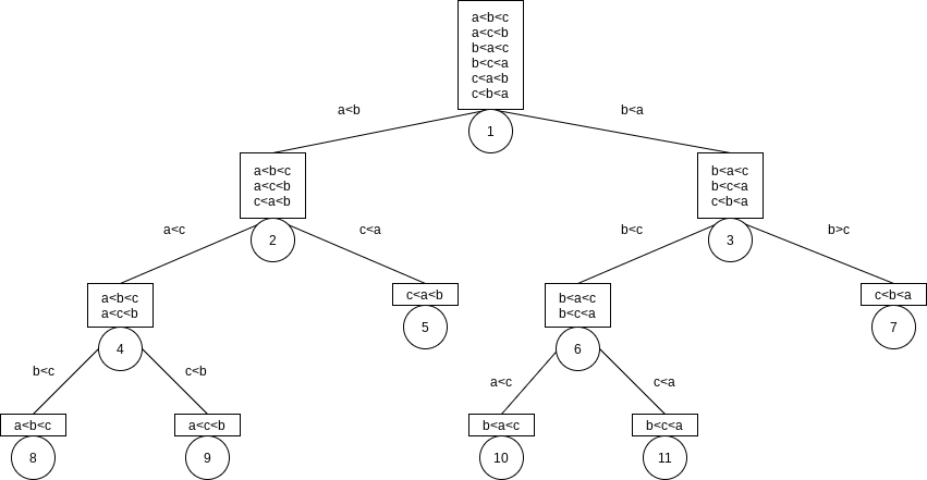
Every algorithm that sorts by using only comparisons can be represented by a decision tree. The number of comparisons used by the sorting algorithm is equal to the depth of the deepest leaf.

Lemma 7.1.

Let be a binary tree of depth . Then has at most leaves.

Lemma 7.2.

A binary tree with leaves must have depth at least .

Theorem 7.6.

Any sorting algorithm that uses only comparisons between elements requires at least comparisons in the worst case.

Proof.

A decision tree to sort elements must have leaves.

Theorem 7.7.

Any sorting algorithm that uses only comparisons between elements requires comparisons.

Proof.

This type of lower-bound argument, when used to prove a worst-case result, is sometimes known as an information-theoretic lower bound.

Note that is roughly .

7.9 Decision-Tree Lower Bounds for Selection Problems

In this section we show additional lower bounds for selection in an N-element collection, specifically

comparisons are necessary to find the smallest item
comparisons are necessary to find the two smallest items
comparisons are necessary to find the median

Lemma 7.3.

If all the leaves in a decision tree are at depth or higher, the decision tree must have at least leaves.

Theorem 7.8.

Any comparison-based algorithm to find the smallest element must use at least comparisons.

Lemma 7.4.

The decision tree for finding the smallest of elements must have at least leaves.

Lemma 7.5.

The decision tree for finding the th smallest of elements must have at least leaves.

Theorem 7.9.

Any comparison-based algorithm to find the th smallest element must use at least comparisons.

Theorem 7.10.

Any comparison-based algorithm to find the second smallest element must use at least comparisons.

Theorem 7.11.

Any comparison-based algorithm to find the median must use at least comparisons.

7.11 Linear-Time Sorts: Bucket Sort and Radix Sort

For bucket sort to work, extra information must be available. The input must consist of only positive integers smaller than . Keep an array called , of size , which is initialized to all 0’s. Thus, has cells, or buckets, which are initially empty. When is read, increment by . After all the input is read, scan the array, printing out a representation of the sorted list. This algorithm takes .

The running time of radix sort is where is the number of passes, is the number of elements to sort, and is the number of buckets.

INITIAL ITEMS:	008	216	512	027	729	000	001	343	125
SORTED BY 1’s digit	001	512	343	064	125	216	027	008	729
SORTED BY 10’s digit:	001	008	512	216	125	027	729	343	064
SORTED BY 100’s digit:	001	008	027	064	125	216	343	512	729

Counting radix sort is an alternative implementation of radix sort that avoids using ArrayLists. Instead, we maintain a count of how many items would go in each bucket; this information can go into an array , so that is the number of items that are in bucket . Then we can use another array , so that represents the number of items whose value is strictly smaller than . Then when we see a value for the first time in the final scan, tells us a valid array spot where it can be written to (but we have to use a temporary array for the write), and after that is done, can be incremented. Counting radix sort thus avoids the need to keep lists. As a further optimization, we can avoid using , by reusing the array. The modification is that we initially have represent the number of items that are in bucket . Then after that information is computed, we can scan the array from the smallest to largest index, and increment by . It is easy to verify that after this scan, the count array stores exactly the same information that would have been stored in offset.

LOADING...

Chapter 7 Sorting

7.2 Insertion Sort

7.2.1 The Algorithm

7.2.2 Analysis of Insertion Sort

7.3 A Lower Bound for Simple Sorting Algorithms

Theorem 7.1.

Proof.

Theorem 7.2.

Proof.

7.4 Shellsort

7.4.1 Worst-Case Analysis of Shellsort

Theorem 7.3.

Proof.

Theorem 7.4.

Proof.

7.5 Heapsort

7.5.1 Analysis of Heapsort

Theorem 7.5.

Proof.

7.6 Mergesort

7.6.1 Analysis of Mergesort

7.7 Quicksort

7.7.1 Picking the Pivot

A Wrong Way

Median-of-Three Partitioning

7.7.3 Small Arrays

7.7.4 Actual Quicksort Routines

7.7.5 Analysis of Quicksort

Worst-Case Analysis

Best-Case Analysis

Average-Case Analysis

7.7.6 A Linear-Expected-Time Algorithm for Selection

7.8 A General Lower Bound for Sorting

7.8.1 Decision Trees

Lemma 7.1.

Lemma 7.2.

Theorem 7.6.

Proof.

Theorem 7.7.

Proof.

7.9 Decision-Tree Lower Bounds for Selection Problems

Lemma 7.3.

Theorem 7.8.

Lemma 7.4.

Lemma 7.5.

Theorem 7.9.

Theorem 7.10.

Theorem 7.11.

7.11 Linear-Time Sorts: Bucket Sort and Radix Sort