Chapter 5 Hashing

5.1 General Idea

Generally a search is performed on some part (that is, data field) of the item. This is called the key. We will refer to the table size as TableSize, with the understanding that this is part of a hash data structure and not merely some variable floating around globally. The common convention is to have the table run from 0 to TableSize - 1.

Each key is mapped into some number in the range 0 to TableSize - 1 and placed in the appropriate cell. The mapping is called a hash function, which ideally should be simple to compute and should ensure that any two distinct keys get different cells. Since there are a finite number of cells and a virtually inexhaustible supply of keys, this is clearly impossible, and thus we seek a hash function that distributes the keys evenly among the cells.

This is the basic idea of hashing. The only remaining problems deal with choosing a function, deciding what to do when two keys hash to the same value (this is known as a collision), and deciding on the table size.

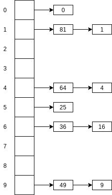
5.3 Separate Chaining

Separate chaining is to keep a list of all elements that hash to the same value.

We define the load factor, , of a hash table to be the ratio of the number of elements in the hash table to the table size. The average length of a list is . The effort required to perform a search is the constant time required to evaluate the hash function plus the time to traverse the list. In an unsuccessful search, the number of nodes to examine is on average. A successful search requires that about links bet raversed. To see this, notice that the list that is being searched contains the one node that stores the match plus zero or more other nodes. The expected number of “other nodes” in a table of elements and lists is , which is essentially , since is presumed to be large. On average, half the “other nodes” are searched, so combined with the matching node, we obtain an average search cost of nodes. This analysis shows that the table size is not really important, but the load factor is. The general rule for separate chaining hashing is to make the table size about as large as the number of elements expected (in other words, let ).

5.4 Hash Tables Without Linked Lists

Generally, the load factor should be below for a hash table that doesn’t use separate chaining. We call such tables probing hash tables.

5.4.1 Linear Probing

In linear probing, is a linear function of , typically . This amounts to trying cells sequentially (with wraparound) in search of an empty cell.

As long as the table is big enough, a free cell can always be found, but the time to do so can get quite large. Worse, even if the table is relatively empty, blocks of occupied cells start forming. This effect, known as primary clustering, means that any key that hashes into the cluster will require several attempts to resolve the collision, and then it will add to the cluster.

It can be shown that the expected number of probes using linear probing is roughly for insertions and unsuccessful searches, and for successful searches. The calculations are somewhat involved.

The corresponding formulas, if clustering is not a problem, are fairly easy to derive. We will assume a very large table and that each probe is independent of the previous probes. These assumptions are satisfied by a random collision resolution strategy and are reasonable unless is very close to . First, we derive the expected number of probes in an unsuccessful search. This is just the expected number of probes until we find an empty cell. Since the fraction of empty cells is , the number of cells we expect to probe is . The number of probes for a successful search is equal to the number of probes required when the particular element was inserted. When an element is inserted, it is done as a result of an unsuccessful search. Thus, we can use the cost of an unsuccessful search to compute the average cost of a successful search.

The caveat is that changes from to its current value, so that earlier insertions are cheaper and should bring the average down. We can estimate the average by using an integral to calculate the mean value of the insertion time, obtaining:

These formulas are clearly better than the corresponding formulas for linear probing. Clustering is not only a theoretical problem but actually occurs in real implementations.

If , then the formula above indicates that probes are expected for an insertion in linear probing. If , then probes are expected, which is unreasonable.

5.4.2 Quadratic Probing

Quadratic probing is a collision resolution method that eliminates the primary clustering problem of linear probing. Quadratic probing is what you would expect – the collision function is quadratic. The popular choice is .

For linear probing it is a bad idea to let the hash table get nearly full, because performance degrades. For quadratic probing, the situation is even more drastic: There is no guarantee of finding an empty cell once the table gets more than half full, or even before the table gets half full if the table size is not prime. This is because at most half of the table can be used as alternative locations to resolve collisions.

---

Theorem 5.1.

If quadratic probing is used, and the table size is prime, then a new element can always be inserted if the table is at least half empty.

Proof.

Let the table size, TableSize, be an (odd) prime greater than . We show that the first alternative locations (including the initial location ) are all distinct. Two of these locations are (mod TableSize) and (mod TableSize), where . Suppose, for the sake of contradiction, that these locations are the same, but . Then

Since TableSize is prime, it follows that either or is equal to (mod TableSize). Since and are distinct, the first option is not possible. Since , the second option is also impossible. Thus, the first TableSize / 2 alternative locations are distinct. If at most TableSize / 2 positions are taken, then an empty spot can always be found.

---

If the table is even one more than half full, the insertion could fail (although this is extremely unlikely). Therefore, it is important to keep this in mind. It is also crucial that the table size be prime.

public class QuadraticProbingHashTable<AnyType> {
    private static final int DEFAULT_TABLE_SIZE = 11;
    
    private HashEntry<AnyType>[] array;
    private int currentSize;
    
    public QuadraticProbingHashTable() {
        this(DEFAULT_TABLE_SIZE);
    }
    
    public QuadraticProbingHashTable(int size) {
        allocateArray(size);
        makeEmpty();
    }
    
    private static class HashEntry<AnyType> {
        public AnyType element;
        public boolean isActive;
        
        public HashEntry(AnyType e) {
            this(e.true);
        }
        
        public HashEntry(AnyType e, boolean i) {
            element = e;
            isActive = i;
        }
    }
    
    public void makeEmpty() {
        currentSize = 0;
        for (int i = 0; i < array.length; i++)
            array[i] = null;
    }
    
    private void allocateArray(int arraySize) {
        array = new HashEntry[nextPrime(arraySize)];
    }
    
    public boolean contains(AnyType x) {
        int currentPos = findPos(x);
        return isActive(currentPos);
    }
    
    private int findPos(AnyType x) {
        int offset = 1;
        int currentPos = myhash(x);
        
        while (array[currentPos] != null && !array[currentPos].element.equals(x)) {
            currentPos += offset;
            offset += 2;
            if (currentPos >= array.length)
                currentPos -= array.length;
        }
        
        return currentPos;
    }
    
    private boolean isActive(int currentPos) {
        return array[currentPos] != null && array[currentPos].isActive;
    }
    
    public void insert(AnyType x) {
        int currentPos = findPos(x);
        if (isActive(currentPos))
            return ;
        
        array[currentPos] = new HashEntry<>(x, true);
        
        if (++currentSize > array.length / 2)
            rehash();
    }
    
    public void remove(AnyType x) {
        int currentPos = findPos(x);
        if (isActive(currentPos))
            array[currentPos].isActive = false;
    }
}

Standard deletion cannot be performed in a probing hash table, because the cell might have caused a collision to go past it.

Although quadratic probing eliminates primary clustering, elements that hash to the same position will probe the same alternative cells. This is known as secondary clustering. Secondary clustering is a slight theoretical blemish. Simulation results suggest that it generally causes less than an extra half probe per search.

5.4.3 Double Hashing

For double hashing, one popular choice is . A poor choice of would be disastrous. Thus, the function must never evaluate to zero. It is also important to make sure all cells can be probed.

5.5 Rehashing

Rehashing is to build another table that is about twice as big (with an associated new hash function) and scan down the entire original hash table, computing the new hash value for each (nondeleted) element and inserting it in the new table.

5.6 Hash Tables in the Standard Library

In Java, library types that can be reasonably inserted into a HashSet or as keys into a HashMap already have equals and hashCode defined. In particular the String class has a hashCode. Because the expensive part of the hash table operations is computing the hashCode, the hashCode method in the String class contains an important optimization: Each String object stores internally the value of its hashCode. Initially it is , but if hashCode is invoked, the value is remembered. Thus if hashCode is computed on the same String object a second time, we can avoid the expensive recomputation. This technique is called caching the hash code, and represents another classic time-space tradeoff.

public final class String {
    private int hash = 0;
    
    public int hashCode() {
        if(hash != 0)
            return hash;
        for(int i = 0; i < length(); i++)
            hash = hash * 31 + (int) charAt( i );
        return hash;
    }
}

Caching the hash code works only because Strings are immutable: If the String were allowed to change, it would invalidate the hashCode, and the hashCode would have to be reset back to .

5.7 Hash Tables with Worst-Case O(1) Access

For separate chaining, assuming a load factor of , this is one version of the classic balls and bins problem: Given balls placed randomly (uniformly) in bins, what is the expected number of balls in the most occupied bin? The answer is well known to be , meaning that on average, we expect some queries to take nearly logarithmic time. Similar types of bounds are observed (or provable) for the length of the longest expected probe sequence in a probing hash table.

5.7.1 Perfect Hashing

Suppose, for purposes of simplification, that all items are known in advance. If a separate chaining implementation could guarantee that each list had at most a constant number of items, we would be done. We know that as we make more lists, the lists will on average be shorter, so theoretically if we have enough lists, then with a reasonably high probability we might expect to have no collisions at all!

---

Theorem 5.2.

If balls are placed into bins, the probability that no bin has more than one ball is less than .

Proof.

If a pair of balls are placed in the same bin, we call that a collision. Let be the expected number of collisions produced by any two balls . Clearly the probability that any two specified balls collide is , and thus is , since the number of collisions that involve the pair is either or . Thus the expected number of collisions in the entire table is . Since there are pairs, this sum is . Since the expected number of collisions is below , the probability that there is even one collision must also be below .

---

Of course, using lists is impractical. However, the preceding analysis suggests the following alternative: Use only bins, but resolve the collisions in each bin by using hash tables instead of linked lists. The idea is that because the bins are expected to have only a few items each, the hash table that is used for each bin can be quadratic in the bin size.

As with the original idea, each secondary hash table will be constructed using a different hash function until it is collision free. The primary hash table can also be constructed several times if the number of collisions that are produced is higher than required. This scheme is known as perfect hashing. All that remains to be shown is that the total size of the secondary hash tables is indeed expected to be linear.

---

Theorem 5.3.

If items are placed into a primary hash table containing bins, then the total size of the secondary hash tables has expected value at most .

Proof.

Using the same logic as in the proof of Theorem 5.2, the expected number of pairwise collisions is at most , or . Let be the number of items that hash to position in the primary hash table; observe that space is used for this cell in the secondary hash table, and that this accounts for pairwise collisions, which we will call . Thus the amount of space used for the th secondary hash table is . The total space is then . The total number of collisions is (from the first sentence of this proof); the total number of items is of course , so we obtain a total secondary space requirement of .

---

Thus the probability that the total secondary space requirement is more than is at most (since, otherwise the expected value would be higher than ), so we can keep choosing hash functions for the primary table until we generate the appropriate secondary space requirement. Once that is done, each secondary hash table will itself require only an average of two trials to be collision free. After the tables are built, any lookup can be done in two probes.

Perfect hashing works if the items are all known in advance. There are dynamic schemes that allow insertions and deletions (dynamic perfect hashing).

5.7.2 Cuckoo Hashing

In cuckoo hashing, suppose we have items. We maintain two tables each more than half empty, and we have two independent has functions that can assign each item to a position in each table. Cuckoo hashing maintains the invariant that an item is always stored in one of these two locations.

The cuckoo hashing algorithm itself is simple: To insert a new item x, first make sure it is not already there. We can then use the first hash function and if the (first) table location is empty, the item can be placed.

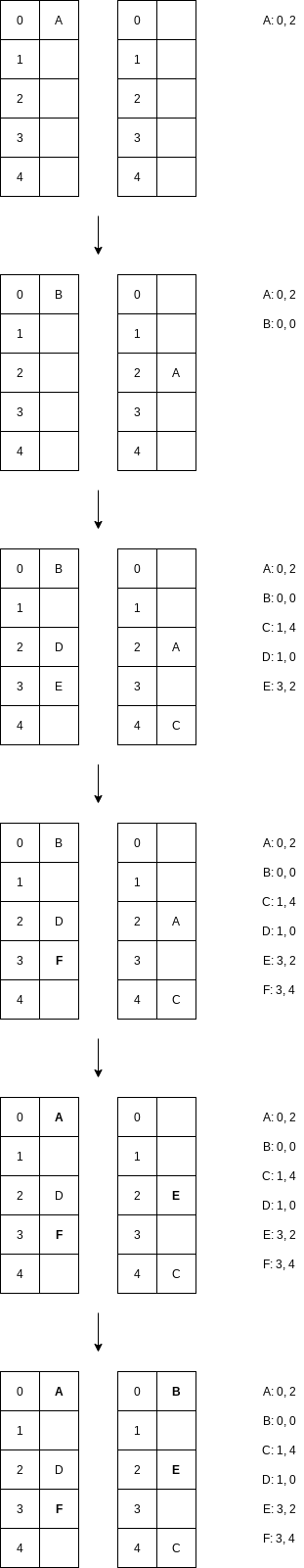
If the table’s load factor is below , an analysis shows that the probability of a cycle is very low, that the expected number of displacements is a small constant, and that it is extremely unlikely that a successful insertion would require more than displacements. As such, we can simply rebuild the tables with new hash functions after a certain number of displacements are detected. More precisely, the probability that a single insertion would require a new set of hash functions can be made to be ; the new hash functions themselves generate more insertions to rebuild the table, but even so, this means the rebuilding cost is minimal.

We cannot successfully insert , with hash locations . At this point, would be in a cycle.

However, if the table’s load factor is at or higher, then the probability of a cycle becomes drastically higher, and this scheme is unlikely to work well at all.

Cuckoo Hash Table Implementation

public interface HashFamily<AnyType> {
    int hash(AnyType x, int which);
    int getNumberOfFunctions();
    void generateNewFunctions();
}

public class StringHashFamily implements HashFamily<String> {
    private final int[] MULTIPLIERS;
    private final java.util.Random r = new java.util.Random();
    
    public StringHashFamily(int d) {
        MULTIPLIERS = new int[d];
        generateNewFunctions();
    }
    
    public int getNumberOfFunctions() {
        return MULTIPLIERS.length;
    }

    public void generateNewFunctions() {
        for(int i = 0; i < MULTIPLIERS.length; i++)
            MULTIPLIERS[i] = r.nextInt();
    }

    public int hash(String x, int which) {
        final int multiplier = MULTIPLIERS[which];
        int hashVal = 0;
        
        for(int i = 0; i < x.length(); i++)
            hashVal = multiplier * hashVal + x.charAt(i);
        
        return hashVal;
    }
}

public class CuckooHashTable<AnyType> {
    private static final double MAX_LOAD = 0.4;
    private static final int ALLOWED_REHASHES = 1;
    private static final int DEFAULT_TABLE_SIZE = 101;
    
    private final HashFamily<? super AnyType> hashFunctions;
    private final int numHashFunctions;
    private AnyType[] array;
    private int currentSize;
    
    private int rehashes = 0;
    private Random r = new Random();
    
    public CuckooHashTable(HashFamily<? super AnyType> hf) {
        this(hf, DEFAULT_TABLE_SIZE);
    }
    
    public CuckooHashTable(HashFamily<? super AnyType> hf, int size) {
        allocateArray(nextPrime(size));
        doClear( );
        hashFunctions = hf;
        numHashFunctions = hf.getNumberOfFunctions();
    }
    
    private void allocateArray(int arraySize) {
        array = (AnyType[])new Object[arraySize];
    }
    
    private void doClear() {
        currentSize = 0;
        for(int i = 0; i < array.length; i++)
            array[ i ] = null;
    }
    
    private int myhash(AnyType x, int which) {
        int hashVal = hashFunctions.hash(x, which);
        hashVal %= array.length;
        if(hashVal < 0)
            hashVal += array.length;
        
        return hashVal;
    }
    
    private int findPos(AnyType x) {
        for(int i = 0; i < numHashFunctions; i++) {
            int pos = myhash(x, i);
            if(array[ pos ] != null && array[pos].equals(x))
                return pos;
        }
        
        return -1;
    }
    
    public boolean contains(AnyType x) {
        return findPos(x) != -1;
    }
    
    public boolean remove(AnyType x) {
        int pos = findPos(x);
        if(pos != -1) {
            array[pos] = null;
            currentSize--;
        }
        
        return pos != -1;
    }
    
    public boolean insert(AnyType x) {
        if(contains(x))
            return false;
        if(currentSize >= array.length * MAX_LOAD)
            expand();
        
        return insertHelper1(x);
    }
    
    private boolean insertHelper1(AnyType x) {
        final int COUNT_LIMIT = 100;
        
        while(true)
        {
            int lastPos = -1;
            int pos;
            
            for(int count = 0; count < COUNT_LIMIT; count++) {
                for(int i = 0; i < numHashFunctions; i++) {
                    pos = myhash(x, i);
                    
                    if(array[pos] == null) {
                        array[pos] = x;
                        currentSize++;
                        return true;
                    }
                }

                int i = 0;
                do {
                    pos = myhash(x, r.nextInt(numHashFunctions));
                } while( pos == lastPos && i++ < 5 );
                
                AnyType tmp = array[lastPos = pos];
                array[pos] = x;
                x = tmp;
            }
            
            if(++rehashes > ALLOWED_REHASHES) {
                expand();
                rehashes = 0;
            } else
                rehash();
        }
    }
    
    private void expand() {
        rehash((int)(array.length / MAX_LOAD));
    }
    
    private void rehash() {
        hashFunctions.generateNewFunctions();
        rehash(array.length);
    }
    
    private void rehash(int newLength) {
        AnyType[] oldArray = array;
        allocateArray(nextPrime(newLength));
        currentSize = 0;
        
        for(AnyType str: oldArray)
            if(str != null)
                insert(str);
    }
}

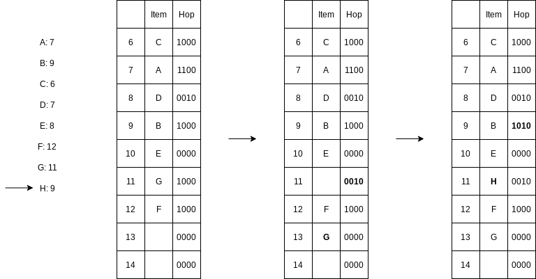
5.7.3 Hopscotch Hashing

Hopscotch hashing is a new algorithm that tries to improve on the classic linear probing algorithm.

The idea of hopscotch hashing is to bound the maximal length of the probe sequence by a predetermined constant that is optimized to the underlying computer’s architecture. Doing so would give constant-time lookups in the worst case, and like cuckoo hashing, the lookup could be parallelized to simultaneously check the bounded set of possible locations.

If an insertion would place a new item too far from its hash location, then we efficiently go backward toward the hash location, evicting potential items. If we are careful, the evictions can be done quickly and guarantee that those evicted are not placed too far from their hash locations. The algorithm is deterministic in that given a hash function, either the items can be evicted or they can’t. The latter case implies that the table is likely too crowded, and a rehash is in order; but this would happen only at extremely high load factors, exceeding 0.9. For a table with a load factor of , the failure probability is almost zero.

Here shows a fairly crowded hopscotch hash table, using MAX_DIST = 4. The bit array for position shows that only position has an item() with hash value : Only the first bit of Hop[6] is set. Hop[7] has the first two bits set, indicating that positions and ( and ) are occupied with items whose hash value . Attempting to insert . Linear probing suggests location , but that is too far, so we evict from position to find a closer position.

5.8 Universal Hashing

Although hash tables are very efficient and have average cost per operation, assuming appropriate load factors, their analysis and performance depend on the hash function having two fundamental properties:

1. The hash function must be computable in constant time.
2. The hash function must distribute its items uniformly among the array slots.

Universal hash functions, which allow us to choose the hash function randomly in such a way that condition 2 above is satisfied.

We use to represent TableSize.

---

Definition 5.1.

A family of hash functions is universal, if for any , the number of hash functions h in for which is at most .

---

---

Definition 5.2.

A family of hash functions is k-universal, if for any , the number of hash functions h in for which , and is at most .

---

To design a simple universal hash function, we will assume first that we are mapping very large integers into smaller integers ranging from to . Let be a prime larger than the largest input key.

---

Theorem 5.4.

The hash family is universal.

Proof.

Let and be distinct values, with , such that .

Clearly if is equal to , then we will have a collision. However, this cannot happen: Subtracting equations yields , which would mean that divides or divides , since is prime. But neither can happen, since both and are between and .

So let and let , and by the above argument, . Thus there are possible values for , and for each , there are possible values for , for a total of possible pairs. Notice that the number of pairs and the number of pairs is identical; thus each pair will correspond to exactly one pair if we can solve for in terms of and . But that is easy: As before, subtracting equations yields , which means that by multiplying both sides by the unique multiplicative inverse of (which must exist, since is not zero and is prime), we obtain , in terms of and . Then follows.

Finally, this means that the probability that and collide is equal to the probability that , and the above analysis allows us to assume that and are chosen randomly, rather than and . Immediate intuition would place this probability at , but that would only be true if were an exact multiple of , and all possible pairs were equally likely. Since is prime, and , that is not exactly true, so a more careful analysis is needed.

For a given , the number of values of that can collide mod is at most (the is because ). It is easy to see that this is at most . Thus the probability that and will generate a collision is at most (we divide by , because as mentioned earlier in the proof, there are only choices for given ). This implies that the hash family is universal.

---

5.9 Extendible Hashing

Extendible hashing, allows a search to be performed in two disk accesses. Insertions also require few disk accesses.

The expected number of leaves is . Thus the average leaf is full. This is the same as for B-trees, which is not entirely surprising, since for both data structures new nodes are created when the th entry is added.

The more surprising result is that the expected size of the directory is . If is very small, then the directory can get unduly large.