Chapter 4 Trees

The data structure that we are referring to is known as a binary search tree. The binary search tree is the basis for the implementation of two library collections classes, TreeSet and TreeMap,

4.1 Preliminaries

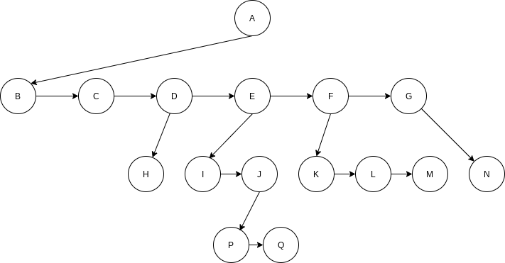
A tree can be defined in several ways. One natural way to define a tree is recursively. A tree is a collection of nodes. The collection can be empty; otherwise, a tree consists of a distinguished node r, called the root, and zero or more nonempty (sub)trees , each of whose roots are connected by a directed edge from .

The root of each subtree is said to be a child of , and is the parent of each subtree root.

Nodes with no children are known as leaves; the leaves in the tree above are , and . Nodes with the same parent are siblings; thus , and are all siblings. Grandparent and grandchild relations can be defined in a similar manner.

A path from node to is defined as a sequence of nodes such that is the parent of for . The length of this path is the number of edges on the path, namely . There is a path of length zero from every node to itself. Notice that in a tree there is exactly one path from the root to each node.

For any node , the depth of is the length of the unique path from the root to . Thus, the root is at depth 0. The height of is the length of the longest path from to a leaf. Thus all leaves are at height 0.

If there is a path from to , then is an ancestor of and is a descendant of . If , then is a proper ancestor of and is a proper descendant of .

4.1.1 Implementation of Trees

One way to implement a tree would be to have in each node, besides its data, a link to each child of the node.

class TreeNode {
    Object element;
    TreeNode firstChild;
    TreeNode nextSibling;
}

4.1.2 Tree Traversals with an Application

In a preorder traversal, work at a node is performed before (pre) its children are processed.

Another common method of traversing a tree is the postorder traversal. In a postorder traversal, the work at a node is performed after (post) its children are evaluated.

4.2 Binary Trees

A property of a binary tree that is sometimes important is that the depth of an average binary tree is considerably smaller than . An analysis shows that the average depth is , and that for a special type of binary tree, namely the binary search tree, the average value of the depth is . Unfortunately, the depth can be as large as .

4.2.1 Implementation

Because a binary tree node has at most two children, we can keep direct links to them.

class BinaryNode {
    Object element;
    BinaryNode left;
    BinaryNode right;
}

4.3 The Search Tree ADT – Binary Search Trees

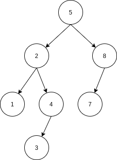
The property that makes a binary tree into a binary search tree is that for every node, , in the tree, the values of all the items in its left subtree are smaller than the item in , and the values of all the items in its right subtree are larger than the item in .

4.3.4 remove

If the node is a leaf, it can be deleted immediately. If the node has one child, the node can be deleted after its parent adjusts a link to bypass the node. The complicated case deals with a node with two children. The general strategy is to replace the data of this node with the smallest data of the right subtree (which is easily found) and recursively delete that node (which is now empty).

4.3.5 Average-Case Analysis

The sum of the depths of all nodes in a tree is known as the internal path length. We will now calculate the average internal path length of a binary search tree, where the average is taken over all possible insertion sequences into binary search trees.

Let be the internal path length for some tree of nodes. . An -node tree consists of an -node left subtree and an -node right subtree, plus a root at depth zero for . is the internal path length of the left subtree with respect to its root. In the main tree, all these nodes are one level deeper. The same holds for the right subtree.

If all subtree sizes are equally likely, which is true for binary search trees (since the subtree size depends only on the relative rank of the first element inserted into the tree), but not binary trees, then the average value of both and is .

If we alternate insertions and deletions times, then the trees will have an expected depth of . After a quarter-million random insert/remove pairs, the tree that was somewhat right-heavy decidedly unbalanced.

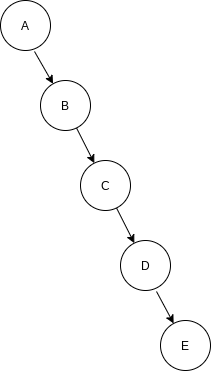
If the input comes into a tree presorted, then a series of inserts will take quadratic time and give a very expensive implementation of a linked list, since the tree will consist only of nodes with no left children. One solution to the problem is to insist on an extra structural condition called balance: No node is allowed to get too deep.

Newer method is to forgo the balance condition and allow the tree to be arbitrarily deep, but after every operation, a restructuring rule is applied that tends to make future operations efficient. These types of data structures are generally classified as self-adjusting. In the case of a binary search tree, we can no longer guarantee an bound on any single operation but can show that any sequence of operations takes total time in the worst case.

4.4 AVL Trees

An AVL (Adelson-Velskii and Landis) tree is a binary search tree with a balance condition. The balance condition must be easy to maintain, and it ensures that the depth of the tree is . The simplest idea is to require that the left and right subtrees have the same height.

Another balance condition would insist that every node must have left and right subtrees of the same height. If the height of an empty subtree is defined to be (as is usual), then only perfectly balanced trees of nodes would satisfy this criterion.

An AVL tree is identical to a binary search tree, except that for every node in the tree, the height of the left and right subtrees can differ by at most .

It can be shown that the height of an AVL tree is at most roughly , but in practice it is only slightly more than .

The minimum number of nodes, , in an AVL tree of height is given by . For , . For , . The function is closely related to the Fibonacci numbers, from which the bound claimed above on the height of an AVL tree follows.

When we do an insertion, we need to update all the balancing information for the nodes on the path back to the root, but the reason that insertion is potentially difficult is that inserting a node could violate the AVL tree property. If this is the case, then the property has to be restored before the insertion step is considered over. It turns out that this can always be done with a simple modification to the tree, known as a rotation.

Let us call the node that must be rebalanced . Since any node has at most two children, and a height imbalance requires that ’s two subtrees’ height differ by two, it is easy to see that a violation might occur in four cases:

1. An insertion into the left subtree of the left child of .
2. An insertion into the right subtree of the left child of .
3. An insertion into the left subtree of the right child of .
4. An insertion into the right subtree of the right child of .

Cases 1 and 4 are mirror image symmetries with respect to , as are cases 2 and 3.

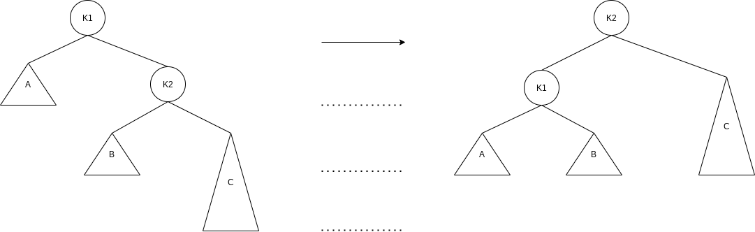
The first case, in which the insertion occurs on the “outside”, is fixed by a single rotation of the tree. The second case, in which the insertion occurs on the “inside” is handled by the slightly more complex double rotation.

4.4.1 Single Rotation

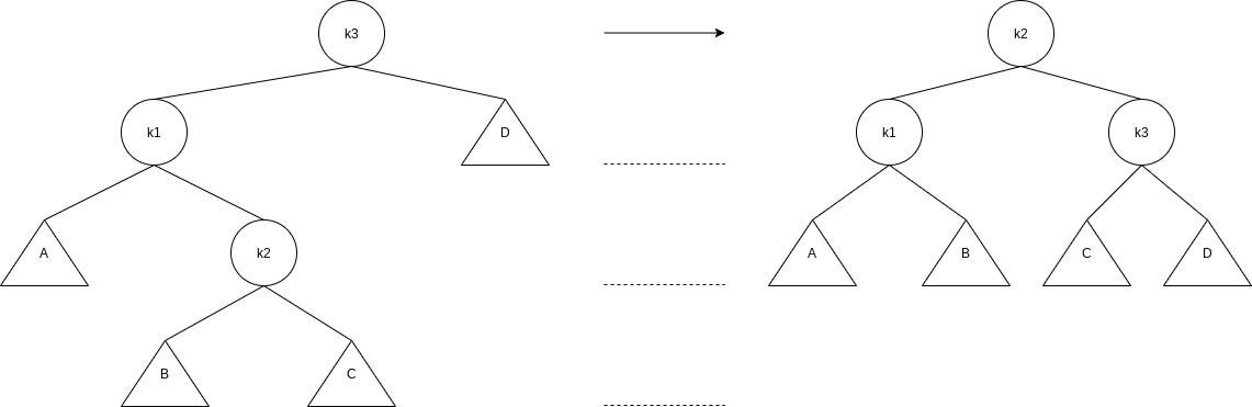
4.4.2 Double Rotation

private static class AvlNode<AnyType> {
    AnyType element;
    AvlNode<AnyType> left;
    AvlNode<AnyType> right;
    int height;
    
    private static final int ALLOWED_IMBALANCE = 1;

    AvlNode(AnyType theElement) {
        this(theElement, null, null);
    }
    
    AvlNode(AnyType theElement, AvlNode<AnyType> lt, AvlNode<AnyType> rt) {
        element = theElement; left = lt; right = rt; height = 0;
    }
    
    private int height(AvlNode<AnyType> t) {
        return t == null ? -1 : t.height;
    }
    
    private AvlNode<AnyType> insert(AnyType x, AvlNode<AnyType> t) {
        if(t == null)
            return new AvlNode<>(x, null, null);
        
        int compareResult = x.compareTo(t.element);
        if( compareResult < 0 )
            t.left = insert(x, t.left);
        else if(compareResult > 0)
            t.right = insert( x, t.right );
        else
            ;
        return balance( t );
    }
    
    private AvlNode<AnyType> remove(AnyType x, AvlNode<AnyType> t) {
        if(t == null)
            return t;
        
        int compareResult = x.compareTo(t.element);
        if(compareResult < 0)
            t.left = remove(x, t.left);
        else if(compareResult > 0)
            t.right = remove( x, t.right );
        else if(t.left != null && t.right != null) {
            t.element = findMin(t.right).element;
            t.right = remove(t.element, t.right);
        } else
            t = (t.left != null) ? t.left : t.right;
        
        return balance( t );
    }

    private AvlNode<AnyType> balance(AvlNode<AnyType> t) {
        if(t == null)
            return t;
        
        if(height(t.left) - height(t.right) > ALLOWED_IMBALANCE)
            if(height(t.left.left) >= height(t.left.right))
                t = rotateWithLeftChild(t);
            else
                t = doubleWithLeftChild(t);
        else if(height(t.right) - height(t.left) > ALLOWED_IMBALANCE)
            if(height(t.right.right) >= height(t.right.left))
                t = rotateWithRightChild(t);
            else
                t = doubleWithRightChild(t);
        
        t.height = Math.max(height(t.left), height(t.right)) + 1;
        return t;
    }
    
    private AvlNode<AnyType> rotateWithLeftChild(AvlNode<AnyType> k2) {
        AvlNode<AnyType> k1 = k2.left;
        k2.left = k1.right;
        k1.right = k2;
        k2.height = Math.max(height(k2.left), height(k2.right)) + 1;
        k1.height = Math.max(height(k1.left), k2.height) + 1;
        return k1;
    }
    
    private AvlNode<AnyType> rotateWithRightChild(AvlNode<AnyType> k2) {
        ...
    }

    private AvlNode<AnyType> doubleWithLeftChild(AvlNode<AnyType> k3) {
        k3.left = rotateWithRightChild(k3.left);
        return rotateWithLeftChild(k3);
    }
    
    private AvlNode<AnyType> doubleWithRightChild(AvlNode<AnyType> k3) {
        ...
    }
}

4.5 Splay Trees

A splay tree guarantees that any consecutive tree operations starting from an empty tree take at most time. Although this guarantee does not preclude the possibility that any single operation might take time, and thus the bound is not as strong as an worst-case bound per operation, the net effect is the same: There are no bad input sequences. Generally, when a sequence of operations has total worst-case running time of , we say that the amortized running time is .

Splay trees are based on the fact that the worst-case time per operation for binary search trees is not bad, as long as it occurs relatively infrequently.

The basic idea of the splay tree is that after a node is accessed, it is pushed to the root by a series of AVL tree rotations.

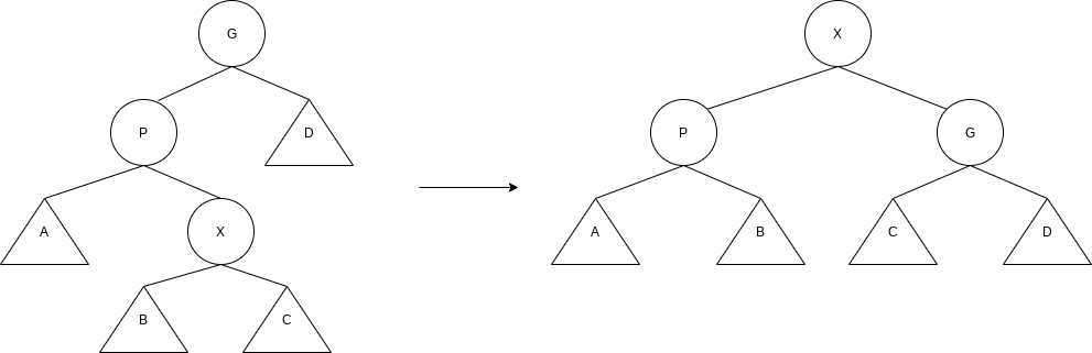
4.5.2 Splaying

Zig-zag

Zig-zig

When accesses are cheap, the rotations are not as good and can be bad. The extreme case is the initial tree formed by the insertions. All the insertions were constant-time operations leading to a bad initial tree.

We can perform deletion by accessing the node to be deleted. This puts the node at the root. If it is deleted, we get two subtrees and (left and right). If we find the largest element in (which is easy), then this element is rotated to the root of , and will now have a root with no right child. We can finish the deletion by making the right child.

4.6 Tree Traversals (Revisited)

Because of the ordering information in a binary search tree, it is simple to list all the items in sorted order. This kind of routine when applied to trees is known as an inorder traversal (which makes sense, since it lists the items in order). The general strategy of an inorder traversal is to process the left subtree first, then perform processing at the current node, and finally process the right subtree. The interesting part about this algorithm, aside from its simplicity, is that the total running time is .

A fourth, less often used, traversal is level-order traversal. In a level-order traversal, all nodes at depth are processed before any node at depth . Level-order traversal differs from the other traversals in that it is not done recursively; a queue is used, instead of the implied stack of recursion.

4.7 B-Trees

Suppose, however, that we have more data than can fit in main memory, meaning that we must have the data structure reside on disk. When this happens, the rules of the game change because the Big-Oh model is no longer meaningful. The problem is that a Big-Oh analysis assumes that all operations are equal. However, this is not true, especially when disk I/O is involved.

An M-ary search tree allows M-way branching. As branching increases, the depth decreases. Whereas a complete binary tree has height that is roughly , a complete M-ary tree has height that is roughly .

We can create an M-ary search tree in much the same way as a binary search tree. In a binary search tree, we need one key to decide which of two branches to take. In an M-ary search tree, we need keys to decide which branch to take. To make this scheme efficient in the worst case, we need to ensure that the M-ary search tree is balanced in some way.

One way to implement this is to use a B-tree. In principle, a B-tree guarantees only a few disk accesses.

A B-tree of order is an M-ary tree with the following properties:

1. The data items are stored at leaves.
2. The nonleaf nodes store up to keys to guide the searching; key represents the smallest key in subtree .
3. The root is either a leaf or has between two and children.
4. All nonleaf nodes (except the root) have between and children.
5. All leaves are at the same depth and have between and data items, for some .