Chapter 12 Advanced Data Structures and Implementation

12.1 Top-Down Splay Trees

We have a current node that is the root of its subtree; this is represented in our diagrams as the “middle” tree. Tree stores nodes in the tree that are less than , but not in ’s subtree; similarly tree stores nodes in the tree that are larger than , but not in ’s subtree. Initially, is the root of , and and are empty.

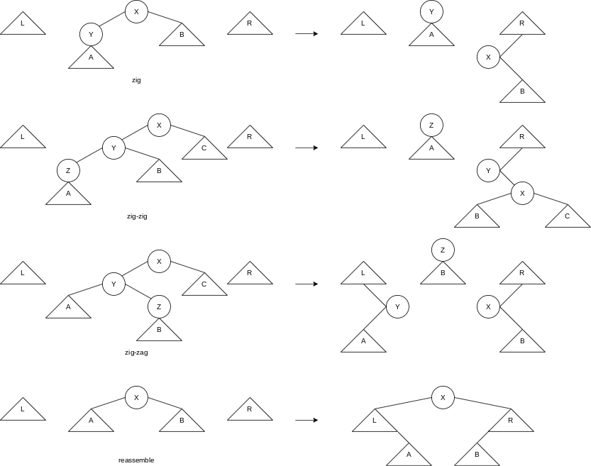
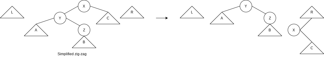
The zig-zag step can be simplified somewhat because no rotations are performed. Instead of making the root of the middle tree, we make the root. The disadvantage is that by descending only one level, we have more iterations in the splaying procedure.

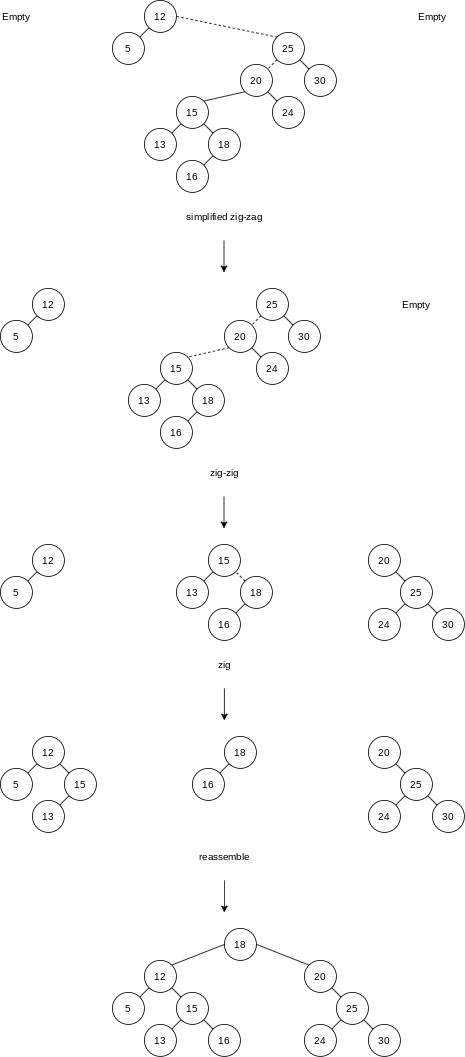
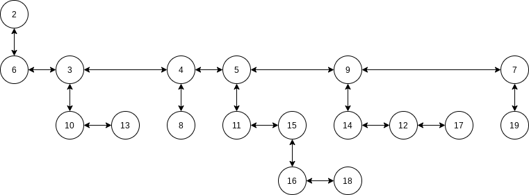
We attempt to access 19 in the tree.

public class SplayTree<AnyType extends Comparable<? super AnyType>> {
    private BinaryNode<AnyType> root;
    private BinaryNode<AnyType> nullNode;
    private BinaryNode<AnyType> header = new BinaryNode<>(null);
    private BinaryNode<AnyType> newNode = null;
    
    public SplayTree() {
        nullNode = new BinaryNode<>(null);
        nullNode.left = nullNode.right = nullNode;
        root = nullNode;
    }
    
    private BinaryNode<AnyType> splay(AnyType x, BinaryNode<AnyType> t) {
        BinaryNode<AnyType> leftTreeMax, rightTreeMin;
        
        header.left = header.right = nullNode;
        leftTreeMax = rightTreeMin = header;
        
        nullNode.element = x;
        
        for (;;)
            if (x.compareTo(t.element) < 0) {
                if (x.compareTo(t.left.element) < 0)
                    t = rotateWithLeftChild(t);
                if (t.left == nullNode)
                    break;
                rightTreeMin.left = t;
                rightTreeMin = t;
                t = t.left
            } else if (x.compareTo(t.element) > 0) {
                if (x.compareTo(t.right.element) > 0)
                    t = rotateWithRightChild(t);
                if (t.right == nullNode)
                    break;
                leftTreeMax.right = t;
                leftTreeMax = t;
                t = t.right;
            } else
                break;
        
        leftTreeMax.right = t.left;
        rightTreeMin.left = t.right;
        t.left = header.right;
        t.right = header.left;
        return t;
    }
    
    public void insert(AnyType x) {
        if (newNode == null)
            newNode = newBinaryNode<>(null);
        newNode.element = x;
        
        if (root == nullNode) {
            newNode.left = newNode.right = nullNode;
            root = newNode;
        } else {
            root = splay(x, root);
            if (x.compareTo(root.element) < 0) {
                newNode.left = root.left;
                newNode.right = root;
                root.left = nullNode;
                root = newNode;
            } else if (x.compareTo(root.element) > 0) {
                newNode.right = root.right;
                newNode.left = root;
                root.right = nullNode;
                root = newNode;
            } else
                return ;
        }
        newNode = null;
    }
    
    public void remove(AnyType x) {
        BinaryNode<AnyType> newTree;
        
        root = splay(x, root);
        if (root.element.compareTo(x) != 0)
            return ;
        
        if (root.left == nullNode)
            newTree = root.right;
        else {
            newTree = root.left;
            newTree = splay(x, newTree);
            newTree.right = root.right;
        }
        root = newTree;
    }
    
    public AnyType findMin() {
        ...
    }
    
    public AnyType findMax() {
        ...
    }
    
    public boolean contains(AnyType x) {
        ...
    }
    
    public void makeEmpty() {
        root = nullNode;
    }
    
    public boolean isEmpty() {
        return root == nullNode;
    }
    
    private BinaryNode<AnyType> rotateWithLeftChild(BinaryNode<AnyType> k2) {
        ...
    }
    
    private BinaryNode<AnyType> rotateWithRightChild(BinaryNode<AnyType> k1) {
        ...
    }
}

12.2 Red-Black Trees

A red-black tree is a binary search tree with the following coloring properties:

1. Every node is colored either red or black.
2. The root is black.
3. If a node is red, its children must be black.
4. Every path from a node to a null reference must contain the same number of black nodes.

A consequence of the coloring rules is that the height of a red-black tree is at most .

The difficulty, as usual, is inserting a new item into the tree. If we color this item black, then we are certain to violate condition , because we will create a longer path of black nodes. Thus the item must be colored red. If the parent is black, we are done. If the parent is already red, then we will violate condition by having consecutive red nodes. In this case, we have to adjust the tree to ensure that condition is enforced. The basic operations that are used to do this are color changes and tree rotations.

12.2.1 Bottom-Up Insertion

If the parent of the newly inserted item is black, we are done.

There are several cases (each with a mirror image symmetry) to consider if the parent is red. First, suppose that the sibling of the parent is black (we adopt the convention that null nodes are black).

Let be the newly added leaf, be its parent, be the sibling of the parent (if it exists), and be the grandparent.

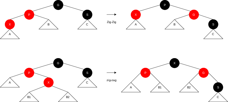
But what happens if S is red? If there is one black node on the path from the subtree’s root to . After the rotation, there must still be only one black node. But in both cases, there are three nodes (the new root, , and ) on the path to . Since only one may be black, and since we cannot have consecutive red nodes, it follows that we’d have to color both and the subtree’s new root red, and black. That’s great, but what happens if the great-grandparent is also red? In that case, we could percolate this procedure up toward the root as is done for B-trees and binary heaps, until we no longer have two consecutive red nodes, or we reach the root (which will be recolored black).

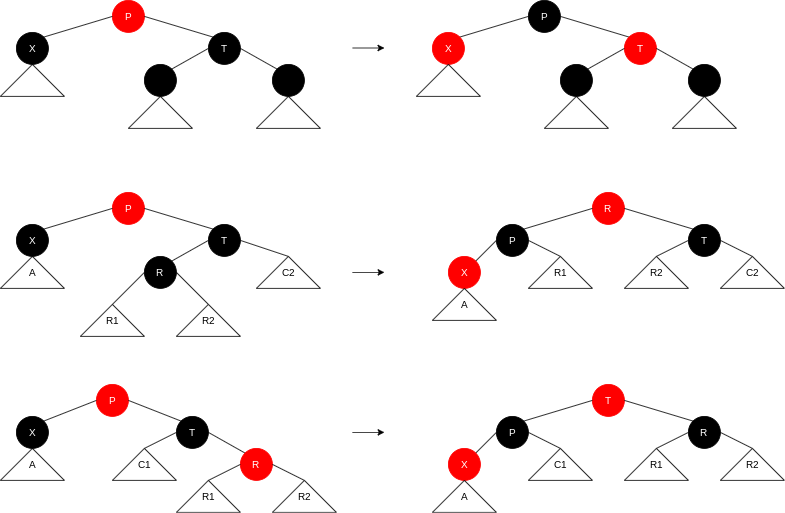
12.2.2 Top-Down Red-Black Trees

We saw that splay trees are more efficient if we use a top-down procedure, and it turns out that we can apply a top-down procedure to red-black trees that guarantees that won’t be red.

The procedure is conceptually easy. On the way down, when we see a node that has two red children, we make red and the two children black. If is the root, after the color flip it will be red but can be made black immediately.

public class RedBlackTree<AnyType extends Comparable<? super AnyType>> {
    private RedBlackNode<AnyType> header;
    private RedBlackNode<AnyType> nullNode;
    
    private static final int BLACK = 1;
    private static final int RED = 0;
    
    private RedBlackNode<AnyType> current;
    private RedBlackNode<AnyType> parent;
    private RedBlackNode<AnyType> grand;
    private RedBlackNode<AnyType> great;
    
    public RedBlackTree() {
        nullNode = new RedBlackNode<>(null);
        nullNode.left = nullNode.right = nullNode;
        header = new RedBlackNode<>(null);
        header.left = header.right = nullNode;
    }
    
    private static class RedBlackNode<AnyType> {
        AnyType element;
        RedBlackNode<AnyType> left;
        RedBlackNode<AnyType> right;
        int color;
        
        RedBlackNode(AnyType theElement) {
            this(thisElement, null, null);
        }
        
        RedBlackNode(AnyType theElement, RedBlackNode<AnyType> lt, RedBlackNode<AnyType rt) {
            element = theElement;
            left = lt;
            right = rt;
            color = RedBlackTree.BLACK;
        }
    }
    
    private RedBlackNode<AnyType> rotate(AnyType item, RedBlackTree<AnyType> parent) {
        if (compare(item, parent) < 0)
            return parent.left = compare(item, parent.left) < 0 ? rotateWithLeftChild(parent.left) : rotateWithRightChild(parent.left);
        else
            return parent.right = compare(item, parent.right) < 0 ? rotateWithLeftChild(parent.right) : rotateWithRightChild(parent.right);
    }
    
    private final int compare(AnyType item, RedBlackNode<AnyType> t) {
        if (t == header)
            return 1;
        else
            return item.compareTo(t.element);
    }
    
    private void handleReorient(AnyType item) {
        current.color = RED;
        current.left.color = BLACK;
        current.right.color = BLACK;
        
        if (parent.color == RED) {
            grand.color = RED;
            if ((compare(item, grand) < 0) != (compare(item, parent) < 0))
                parent = rotate(item, grand);
            current = rotate(item, great);
            current.color = BLACK;
        }
        header.right.color = BLACK;
    }
    
    public void insert(AnyType item) {
        current = parent = grand = header;
        nullNode.element = item;
        
        while (compare(item, current) != 0) {
            great = grand;
            grand = parent;
            parent = current;
            
            current = compare(item, current) < 0 ? current.left : current.right;
            if (current.left.color == RED && current.right.color == RED)
                handleReorient(item);
        }
        
        if (current != nullNode)
            return ;
        current = new RedBlackNode<>(item, nullNode, nullNode);
        
        if (compare(item, parent) < 0)
            parent.left = current;
        else
            parent.right = current;
        handleReorient(item);
    }
    
    public void printTree() {
        if (isEmpty())
            System.out.println("Empty tree");
        else
            printTree(header.right);
    }
    
    public void printTree(RedBlackNode<AnyType> t) {
        if (t != nullNode) {
            printTree(t.left);
            System.out.println(t.element);
            printTree(t.right);
        }
    }
}

12.2.3 Top-Down Deletion

Deletion in red-black trees can also be performed top-down. Everything boils down to being able to delete a leaf. This is because to delete a node that has two children, we replace it with the smallest node in the right subtree; that node, which must have at most one child, is then deleted. Nodes with only a right child can be deleted in the same manner, while nodes with only a left child can be deleted by replacement with the largest node in the left subtree, and subsequent deletion of that node.

Deletion of a red leaf is, of course, trivial. If a leaf is black, however, the deletion is more complicated because removal of a black node will violate condition . The solution is to ensure during the top-down pass that the leaf is red.

Let be the current node, be its sibling, and be their parent. We begin by coloring the root sentinel red. As we traverse down the tree, we attempt to ensure that is red.

First, suppose has two black children. Then there are three subcases.

Otherwise, one of ’s children is red. In this case, we fall through to the next level, obtaining new and . If we’re lucky, will land on the red child, and we can continue onward. If not, we know that will be red, and and will be black. We can rotate and , makeing ’s new parent red; and its grandparent will, of course, be black.

12.3 Treaps

Each node in the tree stores an item, a left and right link, and a priority that is randomly assigned when the node
is created. A treap is a binary search tree with the property that the node priorities satisfy heap order: Any node’s priority must be at least as large as its parent’s.

12.4 Suffix Arrays and Suffix Trees

Suffix array and suffix tree sounds like two data structures, but as we will see, they are basically equivalent, and trade time for space.

12.4 Suffix Arrays and Suffix Trees

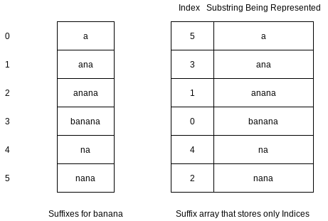
A suffix array for a text is simply an array of all suffixes of arranged in sorted order.

If is a prefix of some substring, it is a prefix of the larger value found at the end of the binary search. Immediately, this reduces the query time to , where the is the binary search, and the is the cost of the comparison at each step.

We can also use the suffix array to find the number of occurrences of : They will be stored sequentially in the suffix array, thus two binary searches suffix to find a range of suffixes that will be guaranteed to begin with . One way to speed this search is to compute the longest common prefix (LCP) for each consecutive pair of substrings; if this computation is done as the suffix array is built, then each query to find the number of occurrences of can be sped up to although this is not obvious.

public static int computeLCP(String s1, String s2) {
    int i = 0;
    while (i < s1.length() && i < s2.length() && s1.charAt(i) == s2.charAt(i))
        i++;
    return i;
}

public static void createSuffixArray(String str, int[] SA, int[] LCP) {
    if (SA.length != str.length() | LCP.length != str.length())
        throw new IllegalArgumentException();
    
    int N = str.length();
    
    String[] suffixes = new String[N];
    for (int i = 0; i < N; i++)
        suffixes[i] = str.substring(i);
    
    Arrays.sort(suffixes);
    
    for (int i = 0; i < N; i++)
        SA[i] = N - suffixes[i].length();
    
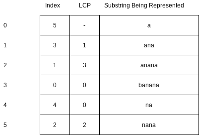
    LCP[0] = 0;
    for (int i = 1; i < N; i++)
        LCP[i] = computeLCP(suffixes[i - 1], suffixes[i]);
}

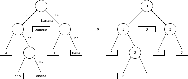
12.4.2 Suffix Trees

Suffix arrays are easily searchable by binary search, but the binary search itself automatically implies cost. What we would like to do is find a matching suffix even more efficiently. One idea is to store the suffixes in a trie.

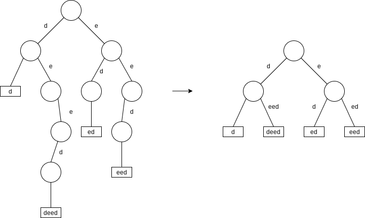
This representation could waste significant space if there are many nodes that have only one child. We see an equivalent representation on the right, known as a compressed trie. Notice that although the branches now have multicharacter labels, all the labels for the branches of any given node must have unique first characters. Thus it is still just as easy as before to choose which branch to take. Thus we can see that a search for a pattern depends only on the length of the pattern , as desired.

If the original string has length , the total number of branches is less than . However, this by itself does not mean that the compressed trie uses linear space: The labels on the edges take up space. And of course writing all the suffixes in the leaves could take quadratic space. So if the original used quadratic space, so does the compressed trie.

1. In the leaves, we use the index where the suffix begins (as in the suffix array).
2. In the internal nodes, we store the number of common characters matched from the root until the internal node; this number represents the letter depth.

In fact, this analysis makes clear that a suffix tree is equivalent to a suffix array plus an LCP array.

At that time we can compute the LCP as follows: If the suffix node value PLUS the letter depth of the parent is equal to , then use the letter depth of the grandparent as the LCP; otherwise use the parent’s letter depth as the LCP.

12.4.3 Linear-Time Construction of Suffix Arrays and Suffix Trees

We describe an worst-case time algorithm to compute the suffix array. This algorithm makes use of divide and conquer. The basic idea is as follows:

1. Choose a sample of suffixes.
2. Sort the sample by recursion.
3. Sort the remaining suffixes, , by using the now-sorted sample of suffixes .
4. Merge and .

We adopt the following conventions:

• : represents the th character of string
• : represents the suffix of starting at index
• : represents an array

Step 1

Sort the characters in the string, assigning them numbers sequentially starting at .

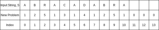
Step 2

Divide the text into three groups:

The idea is that each of consists of roughly symbols, but the symbols are no longer the original alphabet, but instead each new symbol is some group of three symbols from the original alphabet. We will call these tri-characters. Most importantly, the suffixes of combine to form the suffixes of . Thus one idea would be to recursively compute the suffixes of (which by definition implicitly represent sorted strings) and then merge the results in linear time. However, since this would be three recursive calls on problems the original size, that would result in an algorithm. So the idea is going to be to avoid one of the three recursive calls, by computing two of the suffix groups recursively and using that information to compute the third suffix group.

] \
S_2 &= [RAC], [ADA], [BRA]
\end{align}
$$

’s suffixes are ], [ACA][DAB][RA], [RA which clearly correspond to the suffixes in the original string .

Step 3

Concatenate and and recursively compute the suffix array. In order to compute this suffix array, we will need to sort the new alphabet of tri-characters. This can be done in linear time by three passes of radix sort, since the old characters were already sorted in step 1. If in fact all the tri-characters in the new alphabet are unique, then we do not even need to bother with a recursive call. Making three passes of radix sort takes linear time. If is the running time of the suffix array construction algorithm, then the recursive call takes time.

], [RAC], [ADA], [BRA]
$$

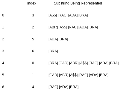
Notice that these are not exactly the same as the corresponding suffixes in ; however, if we strip out characters starting at the first S$, though it is a simple matter to map them back.

Step 4

Compute the suffix array for .

Since our recursive call has already sorted all , we can do step 4 with a simple two-pass radix sort: The first pass is on , and the second pass is on .

From the recursive call in step 3, we can rank the suffixes in and . How the indices in the original string can be referenced from the recursively computed suffix array and shows how the suffix array leads to a ranking of suffixes among .

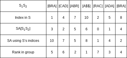
The ranking established in can be used directly for the first radix sort pass on . Then we do a second pass on the single characters from , using the prior radix sort to break ties. Notice that it is convenient if has exactly as many elements as .

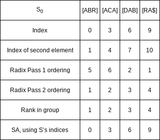
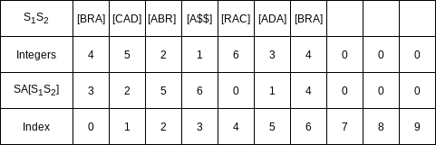
Step 5

Merge the two suffix arrays using the standard algorithm to merge two sorted lists. The only issue is that we must be able to compare each suffix pair in constant time.

The first comparison is between index (an ), which is an element and index (also an ) which is an element. Since that is a tie, we now have to compare index with index . Normally this would have already been computed, since index is , while index is in . However, this is special because index is past the end of the string; consequently it always represents the earlier suffix lexicographically, and the first element in the final suffix array is .

Again the first characters match, so we compare indices and , and and this is already computed, with index having the smaller string.

Once again, the first characters match, so now we have to compare indices and . Since this is a comparison between an element and an element, we cannot look up the result. Thus we have to compare characters directly.

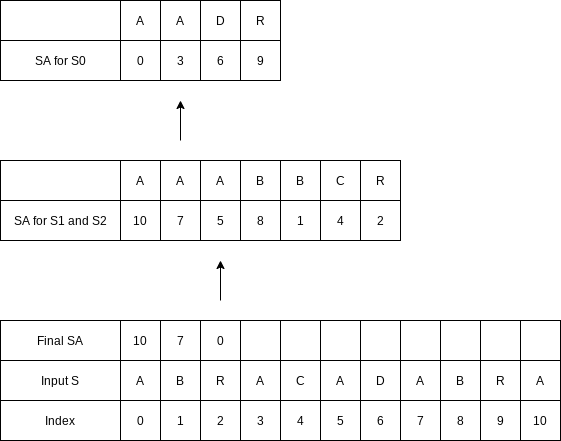
The same situation occurs on the next comparison.

public static void createSuffixArray(String str, int[] sa, int[] LCP) {
    if (sa.length != str.length() || LCP.length != str.length())
        throw new IllegalArgumentException();
    
    int N = str.length();
    
    int[] s = new int[N + 3];
    int[] SA = new int[N + 3];
    
    for (int i = 0; i < N; i++)
        s[i] = str.charAt(i);
    
    makeSuffixArray(s, SA, N, 256);
    
    for (int i = 0; i < N; i++)
        sa[i] = SA[i];
    
    makeLCPArray(s, sa, LCP);
}

public static void makeSuffixArray(int[] s, int[] SA, int n, int K) {
    int n0 = (n + 2) / 3;
    int n1 = (n + 1) / 3;
    int n2 = n / 3;
    int t = n0 - n1;
    int n12 = n1 + n2 + t;
    
    int[] s12 = new int[n12 + 3];
    int[] SA12 = new int[n12 + 3];
    int[] s0 = new int[n0];
    int[] SA0 = new int[n0];
    
    for (int i = 0; j = 0; i < n + t; i++)
        if (i % 3 != 0)
            s12[j++] = i;
    
    int K12 = assignNames(s, s12, SA12, n0, n12, K);
    
    computeS12(s12, SA12, n12, K12);
    computeS0(s, s0, SA0, SA12, n0, n12, K);
    merge(s,s12, SA, SA0, SA12, n, n0, n12, t);
}

private static int assignNames(int[] s, int[] s12, int[] SA12, int n0, int n12, int K) {
    radixPass(s12, SA12, s, 2, n12, K);
    radixPass(SA12, s12, s, 1, n12, K);
    radixPass(s12, SA12, s, 0, n12, K);
    
    int name = 0;
    int c0 = -1, c1 = -1, c2 = -1;
    
    for (int i = 0; i < n12; i++) {
        if (s[SA12[i]] != c0 || s[SA12[i] + 1] != c1 || s[SA12[i] + 2] != c2) {
            name++;
            c0 = s[SA12[i]];
            c1 = s[SA12[i] + 1];
            c2 = s[SA12[i] + 2];
        }
        
        if (SA12[i] % 3 == 1)
            s12[SA12[i] / 3] = name;
        else
            s12[SA12[i] / 3 + n0] = name;
    }
    
    return name;
}

private static void radixPass(int[] in, int[] out, int[] s, int offset, int n, int K) {
    int[] count = new int[K + 2];
    
    for (int i = 0; i < n; i++)
        count[s[in[i] + offset] + 1]++;
    
    for (int i =  1; i <= K + 1; i++)
        count[i] += count[i - 1];
    
    for (int i = 0; i < n; i++)
        out[count[s[in[i] + offset]]++] = in[i];
}

private static void radixPass(int[] in, int[] out, int[] s, int n, int K) {
    radixPass(in, out, s, 0, n, K);
}

private static void computeS12(int[] s12, int[] SA12, int n12, int K12) {
    if (K12 == n12)
        for (int i = 0; i < n12; i++)
            SA12[s12[i] - 1] = i;
    else {
        makeSuffixArray(s12, SA12, n12, K12);
        for (int i = 0; i < n12; i++)
            s12[SA12[i]] = i + 1;
    }
}

private static void computeS0(int[] s, int[] s0, int[] SA0, int[] SA12, int n0, int n12, int K) {
    for (int i = 0, j = 0; i < n12; i++)
        if (SA12[i] < n0)
            s0[j++] = 3 * SA12[i];
    
    radixPass(s0, SA0, s, n0, K);
}

private static void merge(int[] s, int[] s12, int[] SA, int[] SA0, int[] SA12, int n, int n0, int n12, int t) {
    int p = 0, k = 0;
    
    while (t != n12 && p != n0) {
        int i = getIndexIntoS(SA12, t, n0);
        int j = SA0[p];
        
        if (suffix12IsSmaller(s, s12, SA12, n0, i, j, t)) {
            SA[k++] = i;
            t++;
        } else {
            SA[k++] = j;
            p++;
        }
    }
    
    while (p < n0)
        SA[k++] = SA0[p++];
    while (t < n12)
        SA[k++] = getIndexIntoS(SA12, t++, n0);
}

private static int getIndexIntoS(int[] SA12, int t, int n0) {
    if (SA12[t] < n0)
        return SA[t] * 3 + 1;
    else
        return (SA12[t] - n0) * 3 + 2;
}

private static boolean leq(int a1, int a2, int b1, int b2) {
    return a1 < b1 || a1 == b1 && a2 <= b2;
}

private static boolean leq(int a1, int a2, int a3, int b1, int b2, int b3) {
    return a1 < b1 || a1 == b1 && leq(a2, a3, b2, b3);
}

private static boolean suffix12IsSmaller(int[] s, int[] s12, int[] SA12, int n0, int i, int j, int t) {
    if (SA12[t] < n0)
        return leq(s[i], s12[SA12[t] +n0], s[j], s12[j / 3]);
    else
        return leq(s[i]], s[i + 1], s12[SA12[t] - n0 + 1], s[j], s[j + 1], s12[j / 3 + n0]);
}

12.5 -d Trees

The two-dimensional search tree has the simple property that branching on odd levels is done with respect to the first key, and branching on even levels is done with respect to the second key. The root is arbitrarily chosen to be an odd level.

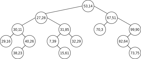
As we go down the tree, we need to maintain the current level. One difficulty is duplicates, particularly since several items can agree in one key.

public void insert(AnyType[] x) {
    root = insert(x, root, 0);
}

private KdNode<AnyType> insert(AnyType[] x, kdNode<AnyType> t, int level) {
    if (t == null)
        t = new KdNode<>(x);
    else if (x[level].compareTo(t.data[level]) < 0)
        t.left = insert(x, t.left, 1 - level);
    else
        t.right = insert(x, t.right, 1 - level);
    return t;
}

A moment’s thought will convince you that a randomly constructed -d tree has the same structural properties as a random binary search tree: The height is on average, but in the worst case.

Unlike binary search trees, for which clever worst-case variants exist, there are no schemes that are known to guarantee a balanced -d tree. The problem is that such a scheme would likely be based on tree rotations, and tree rotations don’t work in -d trees.

We can ask for an exact match, or a match based on one of the two keys; the latter type of request is a partial match query. Both of these are special cases of an (orthogonal) range query.

A range query is easily solved by a recursive tree traversal.

/**
 * low[0] <= x[0] <= high[0] and low[1] <= x[1] <= high[1]
 */
public void printRange(AnyType[] low, AnyType[] high) {
    print(low, high, root, 0);
}

private void printRange(AnyType[] low, AnyType[] high, KdNode<AnyType> t, int level) {
    if (t != null) {
        if (low[0].compareTo(t.data[0]) <= 0 && low[1].compareTo(t.data[1]) <= 0 && high[0].compareTo(t.data[0]) >= 0 && high[1].compareTo(t.data[1]) >= 0)
            System.out.println("(" + t.data[0] + "," + t.data[1] + ")");
        
        if (low[level].compareTo(t.data[level]) <= 0)
            printRange(low, high, t.left, 1 - level);
        if (high[level].compareTo(t.data[level]) >= 0)
            printRange(low, high, t.right, 1 - level);
    }
}

To find a specific item, we can set low equal to high equal to the item we are searching for. To perform a partial match query, we set the range for the key not involved in the match to to .

For a perfectly balanced tree, a range query could take time in the worst case, to report matches. At any node, we may have to visit two of the four grandchildren, leading to the equation . In practice, however, these searches tend to be very efficient, and even the worst case is not poor because for typical , the difference between and is compensated by the smaller constant that is hidden in the Big-Oh notation.

For a randomly constructed tree, the average running time of a partial match query is , where . A recent, and somewhat surprising, result is that this essentially describes the average running time of a range search of a random -d tree.

For dimensions, the same algorithm works; we just cycle through the keys at each level. For a perfectly balanced tree, the worst-case running time of a range query is . In a randomly constructed -d tree, a partial match query that involves of the keys takes , where is the (only) positive root of

12.6 Pairing Heaps

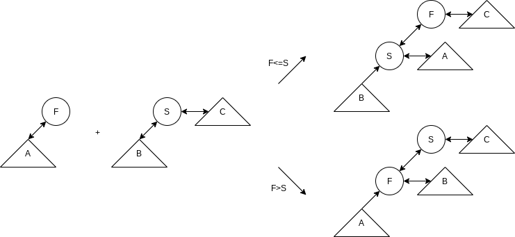
The pairing heap is represented as a heap-ordered tree. The actual pairing heap implementation uses a left child, right sibling representation.

To merge two pairing heaps, we make the heap with the larger root a left child of the heap with the smaller root. Insertion is, of course, a special case of merging. To perform a decreaseKey, we lower the value in the requested node. Because we are not maintaining parent links for all nodes, we don’t know if this violates the heap order. Thus we cut the adjusted node from its parent and complete the decreaseKey by merging the two heaps that result. To perform a deleteMin, we remove the root, creating a collection of heaps. If there are children of the root, then calls to the merge procedure will reassemble the heap. The most important detail is the method used to perform the merge and how the merges are applied.

public class PairingHeap<AnyType extends Comparable<? super AnyType>> {
    private PairNode<AnyType> root;
    private int theSize;
    
    private PairNode<AnyType>[] treeArray = new PairNode[5];
    
    public interface Position<AnyType> {
        AnyType getValue();
    }
    
    private static class PairNode<AnyType> implements Position<AnyType> {
        public AnyType element;
        public PairNode<AnyType> leftChild;
        public PairNode<AnyType> nextSibling;
        public PairNode<AnyType> prev;
        
        public PairNode(AnyType theElement) {
            element = theElement;
            leftChild = nextSibling = prev = null;
        }
        
        public AnyType getValue() {
            return element;
        }
    }
    
    private PairNode<AnyType> compareAndLink(PairNode<AnyType> first, PairNode<AnyType> second) {
        if (second == null)
            return first;

        if (second.element.compareTo(first.element) < 0) {
            second.prev = first.prev;
            first.prev = second;
            first.nextSibling = second.leftChild;
            if (first.nextSibling != null)
                first.nextSibling.prev = first;
            second.leftChild = first;
            return second;
        } else {
            second.prev = first;
            first.nextSibling = second.nextSibling;
            if (first.nextSibling != null)
                first.nextSibling.prev = first;
            second.nextSibling = first.leftChild;
            if (second.nextSibling != null)
                second.nextSibling.prev = second;
            first.leftChild = second;
            return first;
        }
    }
    
    private PairNode<AnyType> combineSiblings(PairNode<AnyType> firstSibling) {
        if (firstSibling.extSibling == null)
            return firstSibling;
        
        int numSiblings = 0;
        for (; firstSibling != null; numSiblings++) {
            treeArray = doubleIfFull(treeArray, numSiblings);
            treeArray[numSiblings] = firstSibling;
            firstSibling.prev.nextSibling = null;
            firstSibling = firstSibling.nextSibling;
        }
        treeArray = doubleIfFull(treeArray, numSiblings);
        treeArray[numSiblings] = null;
        
        int i = 0;
        for (; i + 1 < numSiblings; i += 2)
            treeArray[i] = compareAndLink(treeArray[i], treeArray[i + 1]);
        
        int j = i - 2;
        if (j == numSiblings - 3)
            treeArray[j] = compareAndLink(treeArray[j], treeArray[j + 2]);
        
        for (; j >= 2; j -= 2)
            treeArray[j - 2] = compareAndLink(treeArray[j - 2], treeArray[j]);
        
        return (PairNode<AnyType>) treeArray[0];
    }
    
    private PairNode<AnyType>[] doubleIfFull(PairNode<AnyType>[] array, int index) {
        if (index == array.length) {
            PairNode<AnyType>[] oldArray = array;
            
            array = new PairNode[index * 2];
            
            for (int i = 0; i < index; i++)
                array[i] = oldArray[i];
        }
        
        return array;
    }
    
    public Pisition<AnyType> insert(AnyType x) {
        PairNode<AnyType> newNode = new PairNode<>(x);
        
        if (root == null)
            root = newNode;
        else
            root = compareAndLink(root, newNode);
        
        theSize++;
        return newNode;
    }
    
    public void decreaseKey(Position<AnyType> pos, AnyType newVal) {
        PairNode<AnyType> p = (PairNode<AnyType>) pos;
        
        if (p == null || p.element == null || p.element.compareTo(newVal) < 0)
            throw new IlleagalArgumentException();
        
        p.element = newVal;
        if (p != root) {
            if (p.nextSibling != null)
                p.nextSibling.prev = p.prev;
            if (p.prev.leftChild == p)
                p.prev.leftChild = p.nextSibling;
            else
                p.prev.nextSibling = p.nextSibling;
            
            p.nextSibling = null;
            root = compareAndLink(root, p);
        }
    }
    
    public AnyType deleteMin() {
        if (isEmpty())
            throw new UnderflowException();
        
        AnyType x = findMin();
        root.element = null;
        if (root.leftChild == null)
            root = null;
        else
            root = combineSiblings(root.leftChild);
        
        theSize--;
        return x;
    }
}