Although any operation can still require time, this degenerate behavior cannot occur repeatedly, and we can prove that any sequence of operations takes worst-case time (total). Thus, in the long run this data structure behaves as though each operation takes . We call this an amortized time bound.
11.2 Binomial Queues
Claim.
A binomial queue of elements can be built by successive insertions in time.
Proof.
To prove the claim, we could do a direct calculation. To measure the running time, we define the cost of each insertion to be one time unit plus an extra unit for each linking step. Summing this cost over all insertions gives the total running time. This total is units plus the total number of linking steps. The st, rd, th and all odd-numbered steps require no linking steps, since there is no present at the time of insertion. Thus, half the insertions require no linking steps. A quarter of the insertions require only one linking step (nd, th, th and so on).
In fact, it is easy to see that, in general, an insertion that costs units results in a net increase of trees in the forest, because a tree is created but all trees are removed. Thus, expensive insertions remove trees, while cheap insertions create trees.
Let be the cost of the th insertion. Let be the number of trees after the th insertion. is the number of trees initially. Then we have the invariant
We then have
If we add all these equations, most of the terms cancel, leaving
Recall that and , the number of trees after the insertions, is certainly not negative, so is not negative. Thus
which proves the claim.
During the buildBinomialQueue routine, each insertion had a worst-case time of , but since the entire routine used at most units of time, the insertions behaved as though each used no more than two units each.
The state of the data struc- ture at any time is given by a function known as the potential. The potential function is not maintained by the program but rather is an accounting device that will help with the analysis. When operations take less time than we have allocated for them, the unused time is “saved” in the form of a higher potential. Here, the potential of the data structure is simply the number of trees.
Once a potential function is chosen, we write the main equation:
Notice that while varies from operation to operation, is stable.
Theorem 11.1.
The amortized running times of deleteMin, and merge are and , respectively, for binomial queues.
Proof.
For merge, assume the two queues have and nodes with and trees, respectively. Let . The actual time to perform the merge is . After the merge, there can be at most trees, so the potential can increase by at most . This gives an amortized bound of . The deleteMin bound follows in a similar manner.
11.3 Skew Heaps
Suppose we have two heaps, and , and there are and nodes on their respective right paths. Then the actual time to perform the merge is proportional to , so we will drop the Big-Oh notation and charge one unit of time for each node on the paths.
What is needed is some sort of a potential function that captures the effect of skew heap operations. Recall that the effect of a merge is that every node on the right path is moved to the left path, and its old left child becomes the new right child.
One idea is to classify nodes as either heavy or light, depending on whether or not the right subtree of any node has more nodes than the left subtree.
Definition 11.1.
A node is heavy if the number of descendants of ’s right subtree is at least half of the number of descendants of , and light otherwise. Note that the number of descendants of a node includes the node itself.
The potential function we will use is the number of heavy nodes in the (collection of) heaps. This seems like a good choice, because a long right path will contain an inordinate number of heavy nodes. Because nodes on this path have their children swapped, these nodes will be converted to light nodes as a result of the merge.
Theorem 11.2.
The amortized time to merge two skew heaps is .
Proof.
Let and be the two heaps, with and nodes respectively. Suppose the right path of has light nodes and heavy nodes, for a total of . Likewise, has light and heavy nodes on its right path, for a total of nodes.
If we adopt the convention that the cost of merging two skew heaps is the total number of nodes on their right paths, then the actual time to perform the merge is . Now the only nodes whose heavy/light status can change are nodes that are initially on the right path (and wind up on the left path), since no other nodes have their subtrees altered.
If a heavy node is initially on the right path, then after the merge it must become a light node. The other nodes that were on the right path were light and may or may not become heavy, but since we are proving an upper bound, we will have to assume the worst, which is that they become heavy and increase the potential. Then the net change in the number of heavy nodes is at most . Adding the actual time and the potential change gives an amortized bound of .
Now we must show that . Since and are the number of light nodes on the original right paths, and the right subtree of a light node is less than half the size of the tree rooted at the light node, it follows directly that the number of light nodes on the right path is at most , which is .
Since the insert and deleteMin operations are basically just merges, they also have amortized bounds.
11.4 Fibonacci Heaps
The Fibonacci heap is a data structure that supports all the basic heap operations in amortized time, with the exception of deleteMin and delete, which take amortized time. It immediately follows that the heap operations in Dijkstra’s algorithm will require a total of time.
Fibonacci heaps generalize binomial queues by adding two new concepts:
A different implementation of decreaseKey
Lazy merging
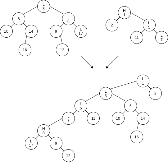
11.4.1 Cutting Nodes in Leftist Heaps
Because we can convert to the leftist heap in steps, and than merge and , we have an algorithm for performing the decreaseKey operation in leftist heaps.
11.4.2 Lazy Merging for Binomial Queues
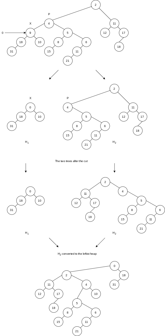
To merge two binomial queues, merely concatenate the two lists of binomial trees, creating a new binomial queue. This new queue may have several trees of the same size, so it violates the binomial queue property. We will call this a lazy binomial queue in order to maintain consistency.
The deleteMin operation is much more painful, because it is where we finally convert the lazy binomial queue back into a standard binomial queue, but, as we will show, it is still amortized time – but not worst-case time, as before.
Amortized Analysis of Lazy Binomial Queues
Theorem 11.3.
The amortized running times of merge and insert are both for lazy binomial queues. The amortized running time of deleteMin is .
Proof.
The potential function is the number of trees in the collection of binomial queues. The initial potential is , and the potential is always nonnegative. Thus, over a sequence of operations, the total amortized time is an upper bound on the total actual time.
For the merge operation, the actual time is constant, and the number of trees in the collection of binomial queues is unchanged, so the amortized time is .
For the insert operation, the actual time is constant, and the number of trees can increase by at most , so the amortized time is .
The deleteMin operation is more complicated. Let be the rank of the tree that contains the minimum element, and let be the number of trees. Thus, the potential at the start of the deleteMin operation is . To perform a deleteMin, the children of the smallest node are split off into separate trees. This creates trees, which must be merged into a standard binomial queue. The actual time to perform this is , if we ignore the constant in the Big-Oh notation, by the argument above. Once this is done, there can be at most trees remaining, so the potential function can increase by at most . Adding the actual time and the change in potential gives an amortized bound of . Since all the trees are binomial trees, we know that .
11.4.3 The Fibonacci Heap Operations
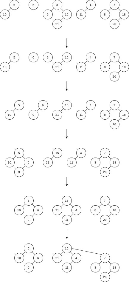
The Fibonacci heap combines the leftist heap decreaseKey operation with the lazy binomial queue merge operation. If arbitrary cuts are made in the binomial trees, the resulting forest will no longer be a collection of binomial trees. Because of this, it will no longer be true that the rank of every tree is at most . Since the amortized bound for deleteMin in lazy binomial queues was shown to be , we need for the deleteMin bound to hold.
In order to ensure that , we apply the following rules to all nonroot nodes:
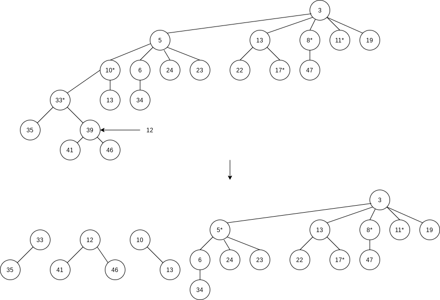
Mark a (nonroot) node the first time that it loses a child (because of a cut).
If a marked node loses another child, then cut it from its parent. This node now becomes the root of a separate tree and is no longer marked. This is called a cascading cut, because several of these could occur in one decreaseKey operation.
11.4.4 Proof of the Time Bound
Lemma 11.1.
Let be any node in a Fibonacci heap. Let be the th oldest child of . Then the rank of is at least .
Proof.
At the time when was linked to , already had (older) children . Thus, had at least children when it linked to . Since nodes are linked only if they have the same rank, it follows that at the time that was linked to , had at least children. Since that time, it could have lost at most one child, or else it would have been cut from . Thus, has at least children.
Lemma 11.2.
Let be the Fibonacci numbers defined by and . Any node of rank has at least descendants (including itself).
Lemma 11.3.
The rank of any node in a Fibonacci heap is .
Theorem 11.4.
The amortized time bounds for Fibonacci heaps are for insert, merge, and decreaseKey and for deleteMin.
Proof.
The potential is the number of trees in the collection of Fibonacci heaps plus twice the number of marked nodes. As usual, the initial potential is and is always nonnegative. Thus, over a sequence of operations, the total amortized time is an upper bound on the total actual time.
For the merge operation, the actual time is constant, and the number of trees and marked nodes is unchanged, so the amortized time is .
For the insert operation, the actual time is constant, the number of trees increases by , and the number of marked nodes is unchanged. Thus, the potential increases by at most , so the amortized time is .
For the deleteMin operation, let be the rank of the tree that contains the minimum element, and let be the number of trees before the operation. To perform a deleteMin, we once again split the children of a tree, creating an additional new trees. Notice that, although this can remove marked nodes (by making them unmarked roots), this cannot create any additional marked nodes. These new trees, along with the other trees, must now be merged, at a cost of . Since there can be at most trees, and the number of marked nodes cannot increase, the potential change is at most . Adding the actual time and potential change gives the amortized bound for deleteMin.
Finally, for the decreaseKey operation, let be the number of cascading cuts. The actual cost of a decreaseKey is , which is the total number of cuts performed. The first (noncascading) cut creates a new tree and thus increases the potential by . Each cascading cut creates a new tree but converts a marked node to an unmarked (root) node, for a net loss of one unit per cascading cut. The last cut also can convert an unmarked node into a marked node, thus increasing the potential by . The total change in potential is thus at most . Adding the actual time and the potential change gives a total of , which is .
11.5 Splay Trees
In order to show an amortized bound for the splaying step, we need a potential function that can increase by at most over the entire splaying step but that will also cancel out the number of rotations performed during the step. It is not at all easy to find a potential function that satisfies these criteria.
A potential function that does work is defined as
where represents the number of descendants of (including itself).
To simplify the notation, we will define
This makes
represents the rank of node . The terminology is similar to what we used in the analysis of the disjoint set algorithm, binomial queues, and Fibonacci heaps. In all these data structures, the meaning of rank is somewhat different, but the rank is generally meant to be on the order (magnitude) of the logarithm of the size of the tree. For a tree with nodes, the rank of the root is simply . Using the sum of ranks as a potential function is similar to using the sum of heights as a potential function. The important difference is that while a rotation can change the heights of many nodes in the tree, only and can have their ranks changed.
Lemma 11.4.
If , and and are both positive integers, then
Theorem 11.5.
The amortized time to splay a tree with root at node is at most .
Proof.
If is the root of , then there are no rotations, so there is no potential change. The actual time is to access the node; thus, the amortized time is and the theorem is true. Thus, we may assume that there is at least one rotation.
For any splaying step, let and be the rank and size of before the step, and let and be the rank and size of immediately after the splaying step.
For the zig step, the actual time is (for the single rotation), and the potential change is . Notice that the potential change is easy to compute, because only ’s and ’s trees change size. Thus, using to represent amortized time,
We see that ; thus, it follows that . Thus,
Since , it follows that , so we may increase the right side, obtaining
For the zig-zag case, the actual cost is , and the potential change is . This gives an amortized time bound of
We see that , so their ranks must be equal. Thus, we obtain
We also see that , Consequently, . Making this substitution gives
We see that . We obtain
Substituting this, we obtain
Since , we obtain
The third case is the zig-zig. The proof of this case is very similar to the zig-zag case.
Since the last splaying step leaves at the root, we obtain an amortized bound of .