
Chapter 10 Algorithm Design Techniques
10.1 Greedy Algorithms
10.1.1 A Simple Scheduling Problem
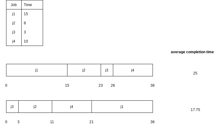
Let the jobs in the schedule be
The first sum is independent of the job ordering, so only the second sum affects the total cost.
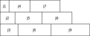
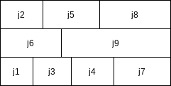
The Multiprocessor Case
The algorithm to solve the multiprocessor case is to start jobs in order, cycling through processors. It is not hard to show that no other ordering can do better, although if the number of processors
Even if
Minimizing the Final Completion Time
Although this schedule does not have minimum mean completion time, it has merit in that the completion time of the entire sequence is earlier. If the same user owns all these jobs, then this is the preferable method of scheduling. Although these problems are very similar, this new problem turns out to be NP-complete; it is just another way of phrasing the knapsack or bin-packing problems. Thus, minimizing the final completion time is apparently much harder than minimizing the mean completion time.
10.1.2 Huffman Codes
| Character | Code | Frequency | Total Bits |
|---|---|---|---|
| a | 000 | 10 | 30 |
| e | 001 | 15 | 45 |
| i | 010 | 12 | 36 |
| s | 011 | 3 | 9 |
| t | 100 | 4 | 12 |
| space | 101 | 13 | 39 |
| newline | 110 | 1 | 3 |
| Total | 174 |
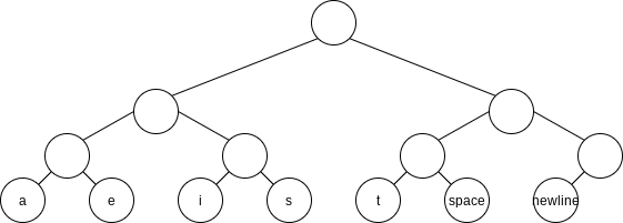
This data structure is sometimes referred to as a trie. If character
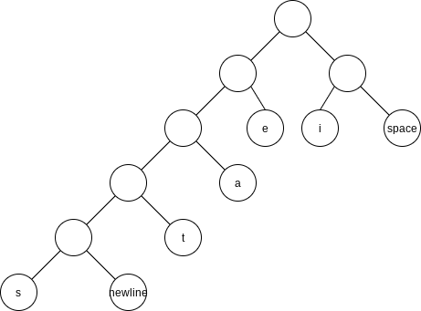
By placing the newline symbol one level higher at its parent, this tree is a full tree: All nodes either are leaves or have two children.
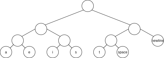
It does not matter if the character codes are different lengths, as long as no character code is a prefix of another character code. Such an encoding is known as a prefix code.
Putting these facts together, we see that our basic problem is to find the full binary tree of minimum total cost, where all characters are contained in the leaves.
| Character | Code | Frequency | Total Bits |
|---|---|---|---|
| a | 001 | 10 | 30 |
| e | 01 | 15 | 30 |
| i | 10 | 12 | 24 |
| s | 00000 | 3 | 15 |
| t | 0001 | 4 | 16 |
| space | 11 | 13 | 26 |
| newline | 00001 | 1 | 5 |
| Total | 146 |
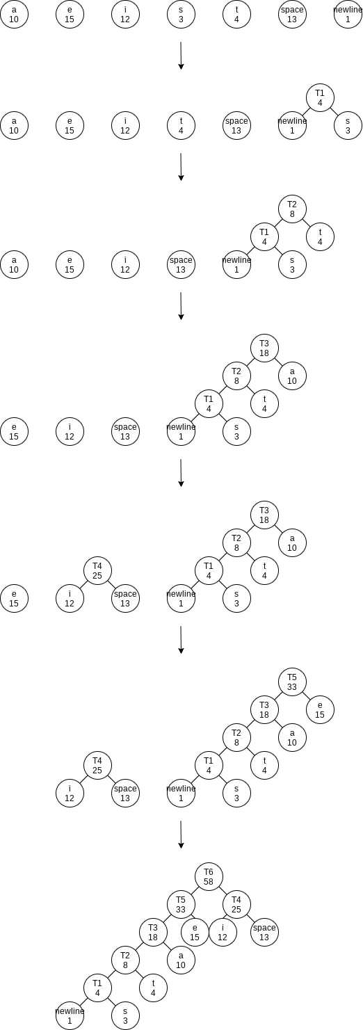
Huffman’s Algorithm
We will assume that the number of characters is
The encoding information must be transmitted at the start of the compressed file, since otherwise it will be impossible to decode. For small files, the cost of transmitting this table will override any possible savings in compression, and the result will probably be file expansion.
The first pass collects the frequency data and the second pass does the encoding. This is obviously not a desirable property for a program dealing with large files.
10.1.3 Approximate Bin Packing
We will consider some algorithms to solve the bin-packing problem. These algorithms will run quickly but will not necessarily produce optimal solutions.
We are given
Online Algorithms
Next Fit
When processing any item, we check to see whether it fits in the same bin as the last item. If it does, it is placed there; otherwise, a new bin is created. This algorithm is incredibly simple to implement and runs in linear time.
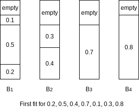
First Fit
The first fit strategy is to scan the bins in order and place the new item in the first bin that is large enough to hold it.
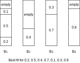
Best Fit
Instead of placing a new item in the first spot that is found, it is placed in the tightest spot among all bins.
Off-line Algorithms
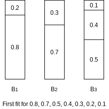
The major problem with all the online algorithms is that it is hard to pack the large items, especially when they occur late in the input. The natural way around this is to sort the items, placing the largest items first. We can then apply first fit or best fit, yielding the algorithms first fit decreasing and best fit decreasing, respectively.
Lemma 10.1.
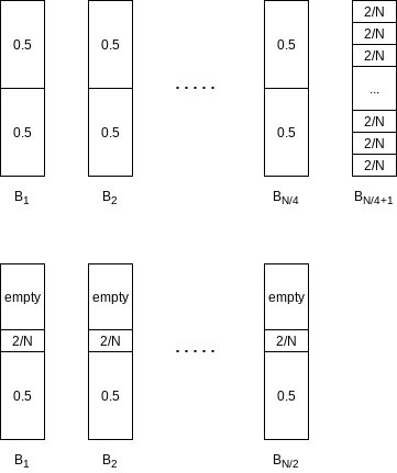
Let the
Proof.
Suppose the
It follows that
Consider the state of the system after the
Suppose there were two bins
To prove the lemma we will show that there is no way to place all the items in
Clearly, no two items
The proof is completed by noting that if
This contradicts the fact that all the sizes can be placed in
Lemma 10.2.
The number of objects placed in extra bins is at most
Proof.
Assume that there are at least
$$
\sum^{N}{i=1}s_i \ge \sum^{M}{j=1}W_j + \sum^{M}{j=1}x_j \ge \sum^{M}{j=1}(W_j + x_j)
$$
Now
$$
\sum^{N}{i=1}s_i > \sum^{M}{j=1}1 > M
$$
But this is impossible if the
10.2 Divide and Conquer
Traditionally, routines in which the text contains at least two recursive calls are called divide-and-conquer algorithms, while routines whose text contains only one recursive call are not. We generally insist that the subproblems be disjoint.
10.2.1 Running Time of Divide-and-Conquer Algorithms
Theorem 10.6.
The solution to the equation
Proof.
We will assume that
If we divide through by
We can apply this equation for other values of
Virtually all the terms on the left cancel the leading terms on the right, yielding
Thus
If
If
Finally, if
As an example, mergesort has
Theorem 10.7.
The solution to the equation
Theorem 10.8.
If
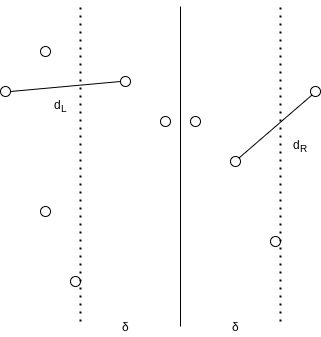
10.2.2 Closest-Points Problem
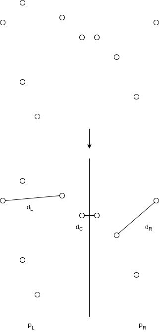
Either the closest points are both in
We can compute
Let
10.2.3 The Selection Problem
Reducing the Average Number of Comparisons
A sample
10.2.4 Theoretical Improvements for Arithmetic Problems
Multiplying Integers
If
Notice that this equation consists of four multiplications,
We see that
Thus, instead of using two multiplications to compute the coefficient of
and so we obtain
Matrix Multiplication
The basic idea of Strassen’s algorithm is to divide each matrix into four quadrants
We could then perform eight
We see that
Strassen used a strategy similar to the integer multiplication divide-and-conquer algorithm and showed how to use only seven recursive calls by carefully arranging the computations. The seven multiplications are
Once the multiplications are performed, the final answer can be obtained with eight more additions.
It is straightforward to verify that this tricky ordering produces the desired values. The running time now satisfies the recurrence
The solution of this recurrence is
As usual, there are details to consider, such as the case when
10.3 Dynamic Programming
Any recursive mathematical formula could be directly translated to a recursive algorithm, but the underlying reality is that often the compiler will not do justice to the recursive algorithm, and an inefficient program results. When we suspect that this is likely to be the case, we must provide a little more help to the compiler, by rewriting the recursive algorithm as a nonrecursive algorithm that systematically records the answers to the subproblems in a table. One technique that makes use of this approach is known as dynamic programming.
10.3.1 Using a Table Instead of Recursion
public static int fib(int n) {
    if (n <= 1)
        return 1;
    else
        return fib(n - 1) + fib(n - 2);
}language-java
Since to compute
public static int fibonacci(int n) {
    if (n <= 1)
        return 1;

    int last = 1;
    int nextToLast = 1;
    int answer = 1;

    for (int i = 2; i <= n; i++) {
        answer = last + nextToLast;
        nextToLast = last;
        last = answer;
    }

    return answer;
}language-java
public static double eval(int n) {
    if (n == 0)
        return 1.0;
    else {
        double sum = 0.0;
        for (int i = 0; i < n; i++)
            sum += eval(i);
        return 2.0 * sum / n + n;
    }
}language-java
The recursive calls duplicate work. In this case, the running time
public static double eval(int n) {
    double[] c = new double[n + 1];

    c[0] = 1.0;
    for (int i = 1; i <= n; i++) {
        double sum = 0.0;
        for (int j = 0; j < i; j++)
            sum += c[j];
        c[i] = 2.0 * sum / i + i;
    }

    return c[n];
}language-java
10.3.2 Ordering Matrix Multiplications
Suppose we are given four matrices,
: multiplications. : multiplications. : multiplications. : multiplications. : multiplications.
It might be worthwhile to perform a few calculations to determine the optimal ordering. Unfortunately, none of the obvious greedy strategies seems to work. Moreover, the number of possible orderings grows quickly. Suppose we define
To see this, suppose that the matrices are
The solution of this recurrence is the well-known Catalan numbers, which grow exponentially. Nevertheless, this counting argument provides a basis for a solution that is substantially better than exponential. Let
Suppose
If we define
This equation implies that if we have an optimal multiplication arrangement of
However, since there are only approximately
public static void optMatrix(int[] c, long[][] m, int[][] lastChange) {
    int n = c.length - 1;

    for (int left = 1; left <= n; left++)
        m[left][left] = 0;
    for (int k = 1; k < n; k++)
        for (int left = 1; left <= n - k; left++) {
            int right = left + k;
            m[left][right] = INFINITY;
            for (int i = left; i < right; i++) {
                long thisCost = m[left][i] + m[i + 1][right] + c[left - 1] * c[i] * c[right];

                if (thisCost < m[left][right]) {
                    m[left][right] = thisCost;
                    lastChange[left][right] = i;
                }
            }
        }
}language-java
10.3.3 Optimal Binary Search Tree
We are given a list of words,
| Word | Probability |
|---|---|
| a | 0.22 |
| am | 0.18 |
| and | 0.20 |
| egg | 0.05 |
| if | 0.25 |
| the | 0.02 |
| two | 0.08 |
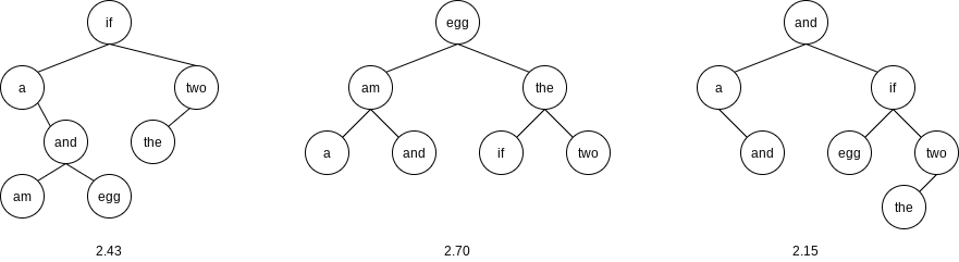
The first tree was formed using a greedy strategy. The word with the highest probability of being accessed was placed at the root. The left and right subtrees were then formed recursively. The second tree is the perfectly balanced search tree. Neither of these trees is optimal, as demonstrated by the existence of the third tree.
This is initially surprising, since the problem appears to be very similar to the construction of a Huffman encoding tree, which, as we have already seen, can be solved by a greedy algorithm. Construction of an optimal binary search tree is harder, because the data are not constrained to appear only at the leaves, and also because the tree must satisfy the binary search tree property.
A dynamic programming solution follows from two observations. Once again, suppose we are trying to place the (sorted) words
If
$$
\begin{align}
C_{Left,Right} &= \min_{Left \le i \le Right} { p_i + C_{Left,i-1} + C_{i+1,Right} + \sum^{i-1}{j=Left}p_j + \sum^{Right}{j=i+1}p_j } \
&= \min_{Left \le i \le Right} { C_{Left,i-1} + C_{i+1,Right} + \sum^{Right}_{j=Left}p_j }
\end{align}
$$
10.3.4 All-Pairs Shortest Path
Dijkstra’s algorithm provides the idea for the dynamic programming algorithm: we select the vertices in sequential order. We will define
When
The time requirement is once again
/**
 * a[][] contains the adjacency matrix with
 * a[i][i] presumed to be zero.
 * d[] contains the values of the shortest path.
 */
public static void allPairs(int[][] a, int[][] d, int[][] path) {
    int n = a.length;

    for (int i = 0; i < n; i++)
        for (int j = 0; j < n; j++) {
            d[i][j] = a[i][j];
            path[i][j] = NOT_A_VERTEX;
        }

    for (int k = 0; k < n; k++)
        for (int i = 0; i < n; i++)
            for (int j = 0; j < n; j++)
                if (d[i][k] + d[k][j] < d[i][j]) {
                    d[i][j] = d[i][k] + d[k][j];
                    path[i][j] = k;
                }
}language-java
10.4 Randomized Algorithms
The worst-case running time of a randomized algorithm is often the same as the worst-case running time of the nonrandomized algorithm. The important difference is that a good randomized algorithm has no bad inputs, but only bad random numbers.
Randomized algorithms were used implicitly in perfect and universal hashing.
10.4.1 Random Number Generators
Actually, true randomness is virtually impossible to do on a computer, since these numbers will depend on the algorithm and thus cannot possibly be random. Generally, it suffices to produce pseudorandom numbers, which are numbers that appear to be random.
The simplest method to generate random numbers is the linear congruential generator, which was first described by Lehmer in 1951. Numbers
To start the sequence, some value of
This sequence has a period of
Lehmer suggested the use of the
It is also common to return a random real number in the open interval
public class Random {
    private static final int A = 48271;
    private static final int M = 2147483647;

    private int state;

    public Random() {
        state = System.currentTimeMillis() % Integer.MAX_VALUE;
    }

    public int randomIntWRONG() {
        return state = (A * state) % M;
    }

    public double random0_1() {
        return (double)randomInt() / M;
    }
}language-java
The problem with this class is that the multiplication could overflow; although this is not an error, it affects the result and thus the pseudorandomness. Schrage gave a procedure in which all the calculations can be done on a
Since
Since
The term
A quick check shows that because
Many libraries have generators based on the function
where
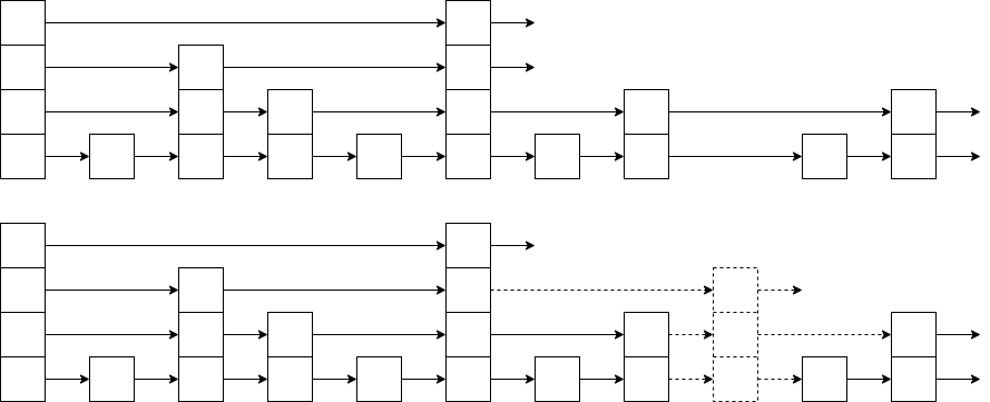
10.4.2 Skip Lists
A linked list in which every other node has an additional link to the node two ahead of it in the list. Because of this, at most
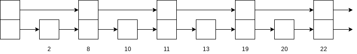
We can extend this idea. Every fourth node has a link to the node four ahead. Only
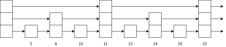
Every
When it comes time to insert a new element, we allocate a new node for it. We must at this point decide what level the node should be. We choose the level of the node randomly, in accordance with this probability distribution.
10.4.3 Primality Testing
Theorem 10.10. (Fermat’s Lesser Theorem)
If
If
We can attempt to randomize the algorithm as follows: Pick
Although this seems to work, there are numbers that fool even this algorithm for most choices of
Theorem 10.11.
If
Proof.
10.5 Backtracking Algorithms
Many other bad arrangements are discarded early, because an undesirable subset of the arrangement is detected. The elimination of a large group of possibilities in one step is known as pruning.
10.5.1 The Turnpike Reconstruction Problem
Suppose we are given
Let
Since

The largest remaining distance is

Since

Now the largest distance is
Since

Once again, so we obtain

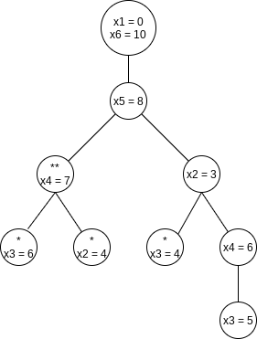
A decision tree representing the actions taken to arrive at the solution. Instead of labeling the branches, we have placed the labels in the branches’ destination nodes. A node with an asterisk indicates that the points chosen are inconsistent with the given distances; nodes with two asterisks have only impossible nodes as children, and thus represent an incorrect path.
boolean turnpike(int[] x, DistSet d, int n) {
    x[1] = 0;
    x[n] = d.deleteMax();
    x[n - 1] = d.deleteMax();
    if (d.contains(x[n] - x[n - 1])) {
        d.remove(x[n] - x[n - 1]);
        return place(x, d, n, 2, n - 2);
    } else
        return false;
}

boolean place(int[] x, DistSet d, int n, int left, int right) {
    int dmax;
    boolean found = false;

    if (d.isEmpty())
        return true;

    dmax = d.findMax();

    // 1 <= j < left && right < j <= n
    if (isRangeExistInD(1, left, d, j -> x[j] - dmax) && isRangeExistInD(right + 1, n + 1, d, j -> x[j] -> dmax)) {
        x[right] = dmax;
        range(1, left).addList(range(right + 1, n + 1)).forEach(j -> d.remove(Math.abs(x[j] - dmax)));
        found = place(x, d, n, left, right - 1);

        if (!found)
            range(1, left).addList(range(right + 1, n + 1)).forEach(j -> d.insert(Math.abs(x[j] - dmax)));
    }

    if (!found && isRangeExistInD(1, left, d, j -> x[n] - dmax - x[j]) && isRangeExistInD(right + 1, n + 1, d, j -> x[n] - dmax - x[j])) {
        x[left] = x[n] - dmax;
        range(1, left).addList(range(right + 1, n + 1)).forEach(j -> d.remove(Math.abs(x[n] - dmax - x[j])));
        found = place(x, d, n, left + 1, right);

        if (!found)
            range(1, left).addList(range(right + 1, n + 1)).forEach(j -> d.insert(Math.abs(x[n] - dmax - x[j])));
    }

    return found;
}language-java
Of course, backtracking happens, and if it happens repeatedly, then the performance of the algorithm is affected. This can be forced to happen by construction of a pathological case. Experiments have shown that if the points have integer coordinates distributed uniformly and randomly from
10.5.2 Games
Minimax Strategy
The more general strategy is to use an evaluation function to quantify the “goodness” of a position. A position that is a win for a computer might get the value of
If a position is not terminal, the value of the position is determined by recursively assuming optimal play by both sides. This is known as a minimax strategy, because one player (the human) is trying to minimize the value of the position, while the other player (the computer) is trying to maximize it.
A successor position of
class MoveInfo {
    public int move;
    public int value;

    public MoveInfo(int m, int v) {
        move = m;
        value = v;
    }
}

class TicTacToe {
    public MoveInfo findCompMove() {
        int i, responseValue;
        int value, bestMove = 1;
        MoveInfo quickWinInfo;

        if (fullBoard())
            value = DRAW;
        else if ((quickWinInfo = immediateCompWin()) != null)
            return quickWinInfo;
        else {
            value = COMP_LOSS;
            for (i = 1; i <= 9; i++)
                if (isEmpty(board(i))) {
                    place(i, COMP);
                    responseValue = findHumanMove().value;
                    unplace(i);

                    if (responseValue > value) {
                        value = responseValue;
                        bestMove = i;
                    }
                }
        }

        return new MoveInfo(bestMove, value);
    }

    public MoveInfo findHumanMove() {
        int i, responseValue;
        int value, bestMove = 1;
        MoveInfo quickWinInfo;

        if (fullBoard())
            value = DRAW;
        else if ((quickWinInfo = immediateHumanWin()) != null)
            return quickWinInfo;
        else {
            value = COMP_WIN;
            for (i = 1; i <= 9; i++) {
                if (isEmpty(board(i))) {
                    place(i, HUMAN);
                    responseValue = findCompMove().value;
                    unplace(i);

                    if (responseValue < value) {
                        value = responseValue;
                        bestMove = i;
                    }
                }
            }
        }

        return new MoveInfo(bestMove, value);
    }
}language-java
The most costly computation is the case where the computer is asked to pick the opening move. Since at this stage the game is a forced draw, the computer selects square
For more complex games, such as checkers and chess, it is obviously infeasible to search all the way to the terminal nodes. In this case, we have to stop the search after a certain depth of recursion is reached.
Nevertheless, for computer chess, the single most important factor seems to be number of moves of look-ahead the program is capable of. This is sometimes known as ply; it is equal to the depth of the recursion.
The basic method to increase the look-ahead factor in game programs is to come up with methods that evaluate fewer nodes without losing any information. One method which we have already seen is to use a table to keep track of all positions that have been evaluated. The data structure that records this is known as a transposition table; it is almost always implemented by hashing.
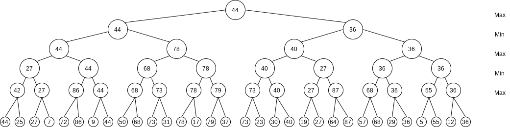
This is commonly referred to as a game tree. We have avoided the use of this term until now, because it is somewhat misleading: No tree is actually constructed by the algorithm. The game tree is just an abstract concept.

Here shows the evaluation of the same game tree, with several (but not all possible) unevaluated nodes. Almost half of the terminal nodes have not been checked. We show that evaluating them would not change the value at the root.
First, consider node findHumanMove and are contemplating a call to findCompMove on findHumanMove will return at most
/**
 * alpha = COMP_LOSS and beta = COMP_WIN
 */
public MoveInfo findCompMove(int alpha, int beta) {
    int i, responseValue;
    int value, bestMove = 1;
    MoveInfo quickWinInfo;

    if (fullBoard())
        value = DRAW;
    else if ((quickWinInfo = immediateCompWin()) != null)
        return quickWinInfo;
    else {
        value = alpha;
        for (i = 1; i <= 9 && value < beta; i++) {
            if (isEmpty(board(i))) {
                place(i, COMP);
                responseValue = findHumanMove(value, beta).value;
                unplace(i);

                if (responseValue > value) {
                    value = responseValue;
                    bestMove = i;
                }
            }
        }
    }

    return new MoveInfo(bestMove, value);
}language-java